Scaling LLM Inference: Data, Pipeline & Tensor Parallelism in vLLM

Introduction

When you chat with ChatGPT or Claude, you're interacting with models that have hundreds of billions to trillions of parameters. These models are so large that they simply cannot fit on a single GPU.

Consider this: an NVIDIA H100 has 80GB of memory. A 70B parameter model in FP16 needs ~140GB just for weights that's nearly 2 H100s worth of memory, and we haven't even counted the KV cache for storing conversation context. For trillion-parameter models like those powering ChatGPT and Claude, you'd need dozens of GPUs just to hold the weights.

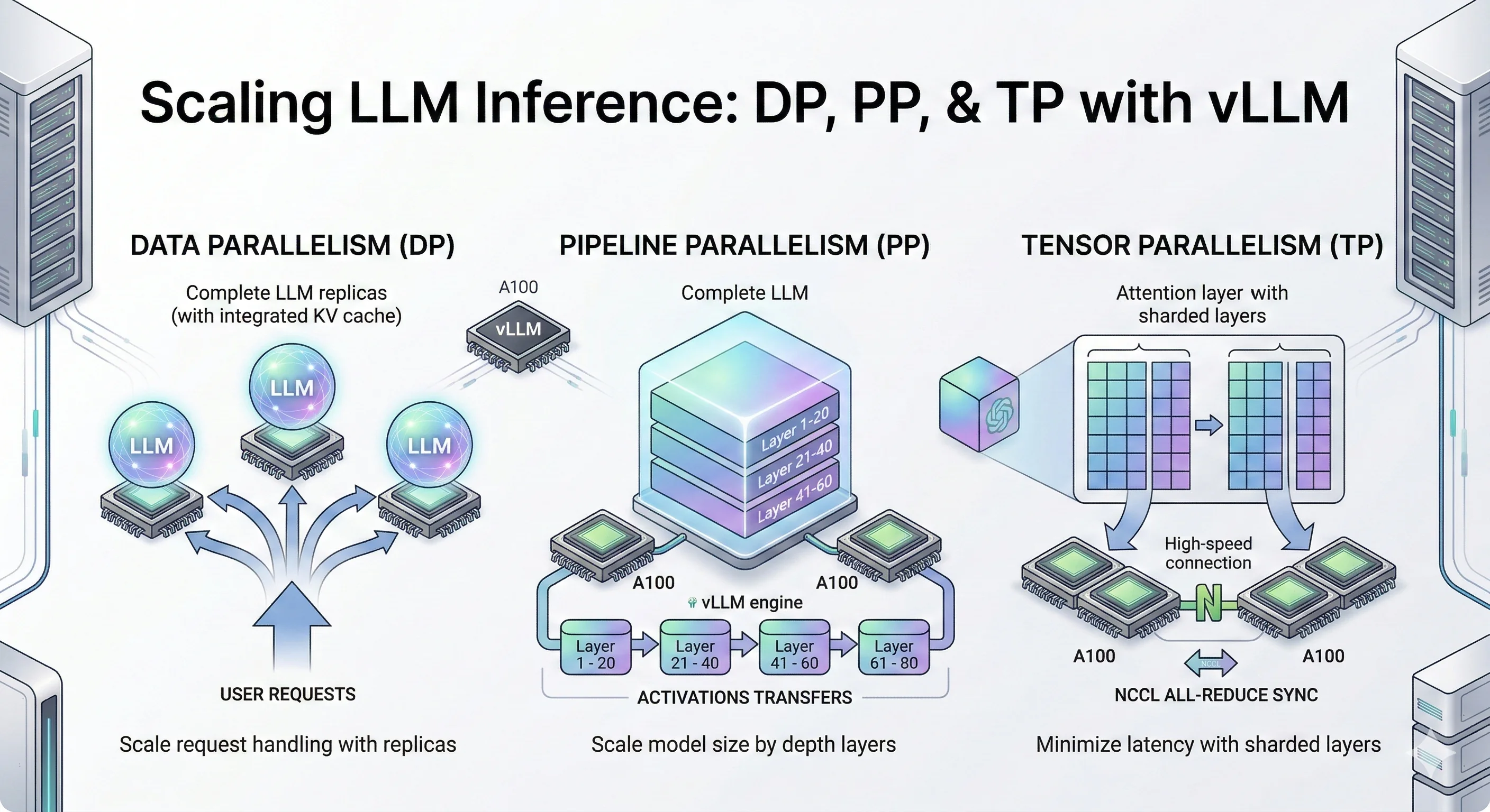
This is where distributed inference comes in — a core challenge in distributed machine learning. Instead of running the entire model on one GPU, we spread the work across multiple GPUs for multi-GPU AI inference at scale. But how exactly do we split a model? There are several strategies — all forms of model parallelism — each with different trade-offs:

Parallelism Strategies Overview

• Data Parallelism (DP), also called data-level parallelism: Make copies of the entire model on multiple GPUs. Each GPU handles different user requests. Simple and effective when your model fits on one GPU but you need more throughput.
• Pipeline Parallelism (PP): Slice the model by layers. GPU 0 runs layers 1-10, GPU 1 runs layers 11-20, and so on. Data flows through GPUs like an assembly line.
• Tensor Parallelism (TP): Split each layer's matrix operations across GPUs. All GPUs work together on the same request, synchronizing after each layer. Best for low latency when you have fast GPU interconnects.
• Expert Parallelism (EP): For Mixture-of-Experts models (like Mixtral), each GPU holds different "expert" sub-networks. Tokens get routed to the right expert. Also called vLLM expert parallelism in the context of vLLM's MoE support.
• Context Parallelism (CP): Split long sequences across GPUs. Each GPU handles a portion of the context, useful for very long prompts.

In this blog, we dive deep into three core LLM inference techniques: Data Parallelism (DP), Pipeline Parallelism (PP), and Tensor Parallelism (TP). These are the foundational LLM inference optimization strategies for vLLM distributed inference and distributed LLM serving that you'll encounter in most LLM serving systems like vLLM, TensorRT-LLM, and SGLang.

We'll cover Expert Parallelism (EP) and Context Parallelism (CP) in future blog posts, along with multi-node distributed inference across machines.

While trillion-parameter models require massive GPU clusters to run, the same parallelism techniques apply to smaller models too. For our experiments, we use Qwen3-32B and Qwen3-14B models small enough to benchmark on a few GPUs, but large enough to demonstrate the real trade-offs between DP, PP, and TP.

Think of these experiments as a scaled-down version of what happens at major AI labs. The principles are identical: when you understand how DP, PP, and TP behave on a 14B/32B model, you understand how they'll behave on a trillion-parameter model just with bigger numbers.

Let's deep dive into each technique.

Key Findings

• Data Parallelism (DP) scales throughput by ~50% at moderate concurrency (c=120–180) with no inter-GPU communication — the simplest LLM optimization for scaling model inference.
• Pipeline Parallelism (PP) enables serving models that don't fit on a single GPU, cutting TTFT P99 by 2.5–3× at high concurrency through larger aggregate KV cache.
• Tensor Parallelism (TP) delivers the best latency across all metrics simultaneously — 3× TTFT improvement, consistent TPOT and ITL gains — but requires fast GPU interconnects (NVLink).
• The key mental model: If you are limited by request volume, use DP. If you are limited by GPU memory, use PP. If you are limited by compute speed and latency, use TP.

What Is Data Parallelism (DP)?

Data Parallelism (DP) replicates the entire model on each GPU and distributes incoming requests across replicas for linear throughput scaling.

Data Parallelism is the simplest way to scale LLM inference. The idea is straightforward instead of making one GPU work harder, you run multiple full copies of the model on different GPUs and split the incoming traffic between them. Each GPU gets its own set of requests, processes them completely independently, and streams back responses. There's no communication between GPUs during inference. They don't know each other exists. If one GPU handles 50 requests/second, adding a second GPU with DP=2 gets you ~100 requests/second. You're not making individual requests faster you're handling more of them simultaneously. DP effectively enables vLLM batch inference across replicas — each replica processes its own batch independently.

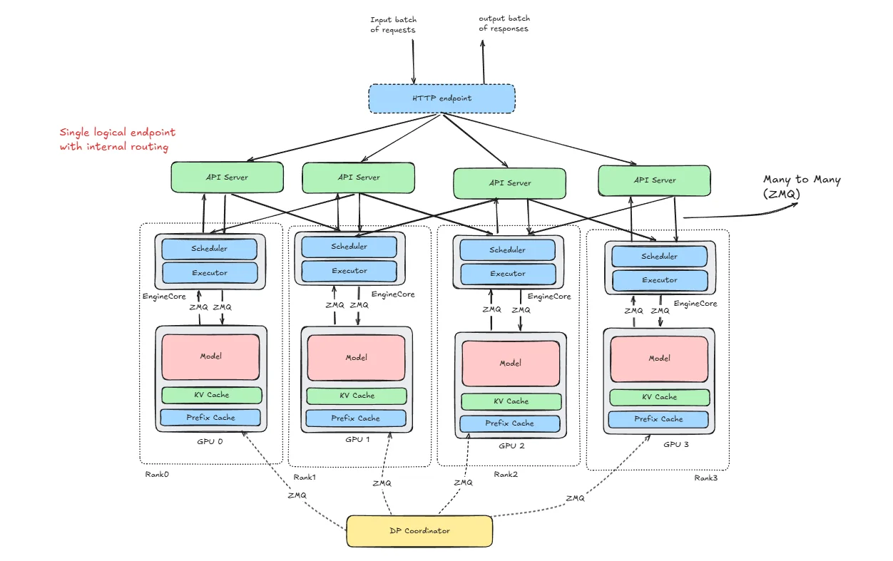
How vLLM Is Structured for DP

To understand how requests flow through the system, let's learn about the key terms first:

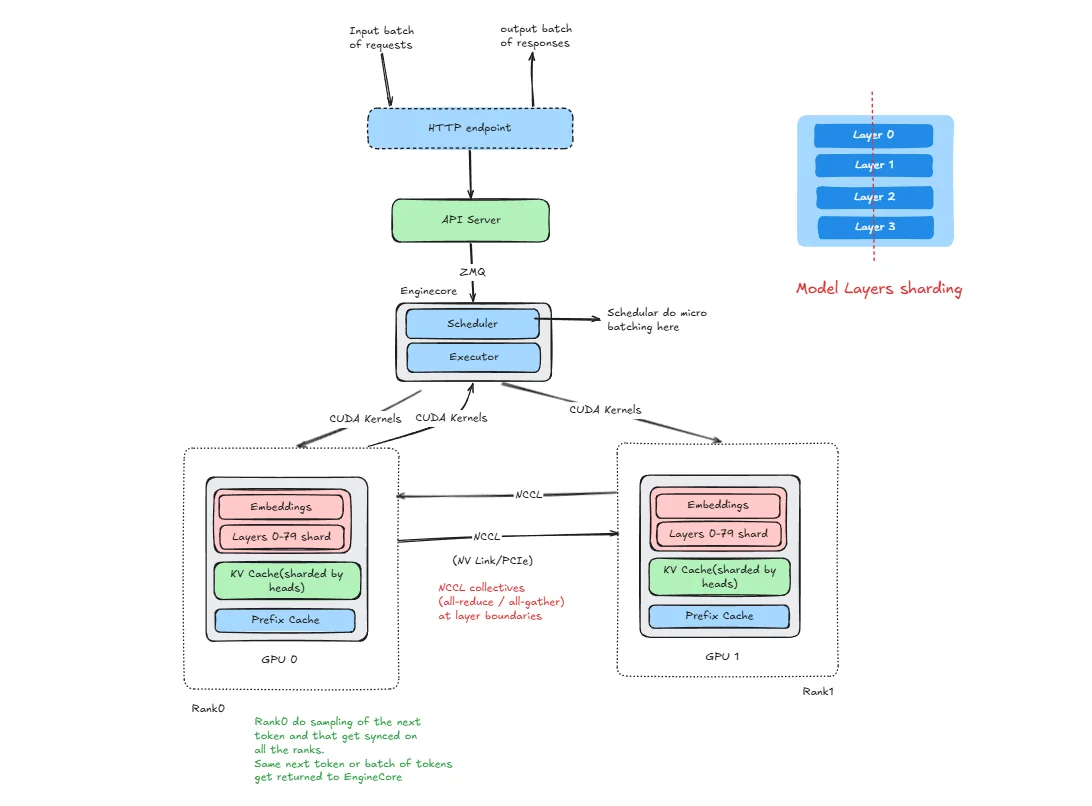
HTTP Endpoint

Just the public entry point. Clients send requests here. It doesn't know anything about GPUs or scheduling. it's just the front door.

API Server

This is where requests first get processed. vLLM does all request preprocessing here: parsing of the requests, tokenization of the prompts, applying generation parameters, and deciding which DP rank should handle it. It does routing, not inference. Any API worker can send a request to any rank.

Rank

A rank is simply one full replica of the model. If DP=4, you have 4 ranks. each rank loads the full model, has its own KV cache, has its own scheduler and ranks do not share KV cache. They are independent.

Engine Core

This is the actual inference engine inside each rank. It manages the scheduler, runs continuous batching, updates KV cache, sends work to the GPU If you think “where does real inference logic live?” this is it.

ZMQ

ZMQ is just the messaging layer between API server ↔ engine cores, DP Coordinator ↔ ranks. It’s not doing compute just passing messages.

DP Coordinator

This one confuses people. It does not run inference. It does not route HTTP requests. It exists to Track rank state, Help with coordination, Handle synchronization (especially for MoE models).

Now let's see how these vLLM components works in case of DP initialization and inference of single request.

---

Initialization

vllm serve Qwen/Qwen3-32B --data-parallel-size 2

When we run this, vLLM launches two engine processes (Rank 0 and Rank 1), each assigned to a GPU. Both ranks load the full model into their GPU memory and allocate their own KV cache. A coordination group is initialized, the scheduler loop starts inside each rank, and the API server begins listening. Now the system is ready to serve.

---

Inference

Let’s say one request comes in.

Step 1 : Request arrives Client → HTTP endpoint → API server.

Step 2 : API server checks which rank is less busy (and possibly cache-aware). It chooses one rank.

Step 3 : Send to engine core. The request is sent via ZMQ to that rank.

Step 4 : Scheduling Inside that rank

• The scheduler queues it.
• It gets batched with other active requests.

Step 5 : The model runs prefill and decode on that GPU. KV cache is updated locally.

Step 6 : Tokens go back to API server → then to client.

Other ranks are not involved in this request.

---

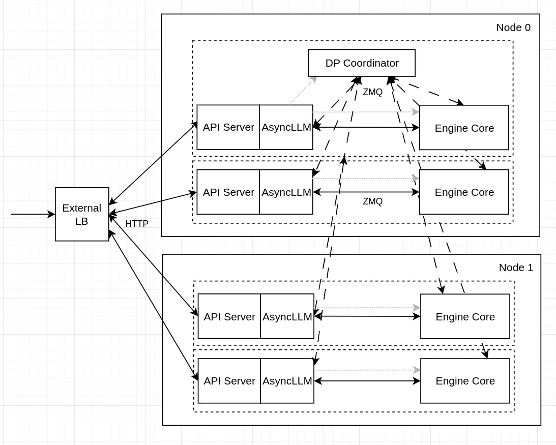
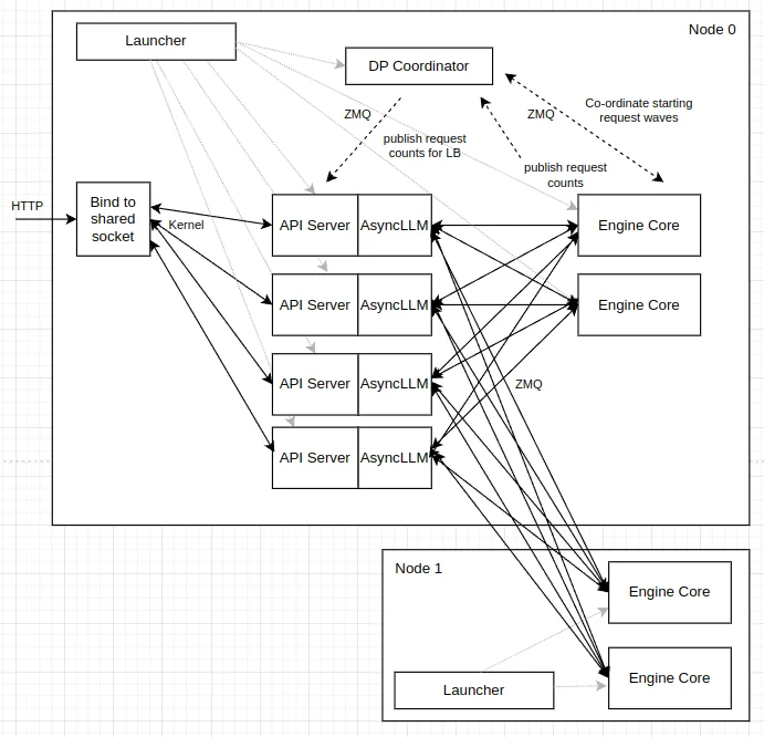
Internal vs External Load Balancing

So far we've seen how a single request gets routed to a rank. But how does your traffic actually reach the vLLM server in the first place? There are two approaches, and they differ in how much visibility the routing layer has into the actual GPU state.

External Load Balancing

Source: https://docs.vllm.ai/en/latest/serving/data_parallel_deployment/#internal-load-balancing

With external load balancing, you run multiple independent vLLM instances and put a load balancer (like nginx or HAProxy) in front of them. Each instance runs on its own GPU and has no idea about the others.

CUDA_VISIBLE_DEVICES=0 vllm serve Qwen/Qwen3-32B --port 8000
CUDA_VISIBLE_DEVICES=1 vllm serve Qwen/Qwen3-32B --port 8001

The load balancer routes incoming requests using simple strategies like round-robin or least-connections. It's easy to set up and each instance is fully isolated — if one crashes, the other keeps running.

The downside is that the load balancer is completely blind to what's happening inside each GPU. It doesn't know how full the KV cache is, whether a rank is in the middle of a heavy prefill batch, or whether one GPU is sitting idle while the other is overloaded.

Internal Load Balancing

Source: https://docs.vllm.ai/en/latest/serving/data_parallel_deployment/#internal-load-balancing

With internal load balancing, vLLM manages everything through a single entry point using the --data-parallel-size flag:

vllm serve Qwen/Qwen3-32B --data-parallel-size 2 --port 8000

Here the API server has direct visibility into each rank's queue state — how many requests are waiting and how many are currently running. This lets it route new requests to the least-loaded rank, keeping both GPUs balanced under bursty traffic. (Future versions may incorporate richer signals such as KV cache pressure and prefill/decode state, but the current implementation uses queue-count-based scoring.)

The trade-off is slightly more complexity and a single point of entry, but for most production setups the smarter routing is worth it.

---

Getting the Hardware

To run the experiments in this blog post you can rent a GPU at JarvisLabs. See our H100 pricing guide or H200 GPU pricing for current costs on multi-GPU setups.

Here's how to set up your own instance:

1. Log in: JarvisLabs and navigate to the dashboard.
2. Create an instance: click Create and select your desired GPU configuration.
3. Select your GPU : choose A100 for higher performance; it is sufficient for all experiments in this blog post.
4. Choose the framework : select PyTorch from the available frameworks.
5. Launch : click Launch. Your instance will be ready in a few minutes.

Benchmarks

Model: Qwen3-32B | GPUs: 2× A100-80GB | Dataset: ShareGPT | Strategy: Data Parallelism

Experiment: Qwen/Qwen3-32B with ShareGPT dataset, comparing with and without DP, run on 2× NVIDIA A100 80GB GPUs.

The server was started with:

# Baseline (no DP)
vllm serve Qwen/Qwen3-32B \
  --dtype bfloat16 \
  --host 0.0.0.0 \
  --gpu-memory-utilization 0.92 \
  --max-model-len 20480 \
  --port 8000

# DP=2
vllm serve Qwen/Qwen3-32B \
  --host 0.0.0.0 \
  --port 8000 \
  --data-parallel-size 2 \
  --dtype bfloat16 \
  --gpu-memory-utilization 0.92 \
  --max-model-len 20480

Each data point in the table below comes from a separate client run, varying only --max-concurrency. First, download the ShareGPT dataset:

wget https://huggingface.co/datasets/anon8231489123/ShareGPT_Vicuna_unfiltered/resolve/main/ShareGPT_V3_unfiltered_cleaned_split.json

Then run the benchmark:

vllm bench serve \
  --model Qwen/Qwen3-32B \
  --dataset-name sharegpt \
  --dataset-path ./ShareGPT_V3_unfiltered_cleaned_split.json \
  --host 127.0.0.1 \
  --port 8000 \
  --max-concurrency 60 \
  --seed 42 \
  --num-prompts 1000

Everything else stays fixed same model, same dataset, same 1,000 prompts, same random seed. The only knob being turned is --max-concurrency, which controls how many requests are in-flight at once. This gives a clean comparison of how each configuration behaves under increasing load.

In the following table each column (c=60 to c=420) is a separate benchmark run with that many concurrent requests. Rows show throughput and tail latency metrics. Higher is better for throughput, lower is better for latency. The key pattern to look for: DP=2 should improve throughput and cut latency, especially as concurrency grows.

Metric	Config	c=60	c=120	c=180	c=240	c=300	c=360	c=420
Output Throughput (tok/s)	Baseline (no DP)	1,556.40	1,797.41	1,781.21	1,907.36	1,784.93	1,907.79	1,897.22
	DP=2	1,801.42	2,526.64	2,833.13	2,723.37	2,349.34	2,798.28	2,379.19
Total Throughput (tok/s)	Baseline (no DP)	3,235.25	3,730.53	3,704.40	3,967.26	3,708.95	3,983.55	3,961.84
	DP=2	3,740.72	5,262.36	5,906.59	5,652.73	4,892.83	5,833.78	4,935.40
TTFT P99 (ms)	Baseline (no DP)	1,461.03	5,641.03	11,020.16	16,866.75	23,002.35	28,096.11	32,634.63
	DP=2	793.83	1,459.79	2,378.73	9,040.82	15,288.21	15,517.01	21,257.14
TPOT P99 (ms)	Baseline (no DP)	43.54	122.17	190.26	127.29	190.10	190.69	158.24
	DP=2	33.46	47.82	71.53	132.13	172.95	170.41	226.65
ITL P99 (ms)	Baseline (no DP)	92.90	137.27	158.20	145.35	139.07	135.35	147.55
	DP=2	66.48	90.09	103.88	112.70	127.23	128.74	123.84

Throughput comparison

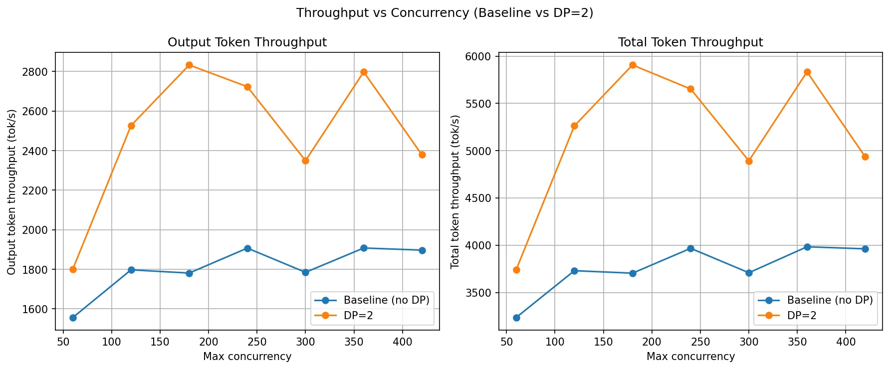
This graph shows how output and total throughput scale as concurrency increases from 60 to 420.

• The baseline throughput jumps from 1,556 tok/s at c=60 to 1,797 at c=120, then essentially stops growing. it oscillates between 1,781 and 1,907 for all remaining concurrency levels. This plateau is the knee point for the baseline. The single GPU is fully saturated by around c=120. Beyond that, adding more requests doesn't produce more tokens. it just builds up a longer queue. You're not getting more throughput, just more waiting.
• DP=2 continues scaling past the baseline's plateau. It rises from 1,801 at c=60 to 2,526 at c=120 and peaks at 2,833 at c=180. That peak is DP=2's knee point. After c=180, the numbers become inconsistent 2,723 at c=240, dropping to 2,349 at c=300, then back up to 2,798 at c=360 and down again at c=420. This oscillation means both GPUs are now approaching saturation and the load balancer is doing its best but can no longer keep both ranks evenly loaded.

The gap between the two curves is the gain we are getting from the second GPU. It's widest at c=120–c=180, which is the ideal operating range for DP=2 on this model and hardware. If your traffic sits in that range, DP=2 gives a clean ~50% throughput boost. Beyond c=300, both configs are memory-bound and throughput gains become unpredictable.

TTFT, TPOT and ITL comparison

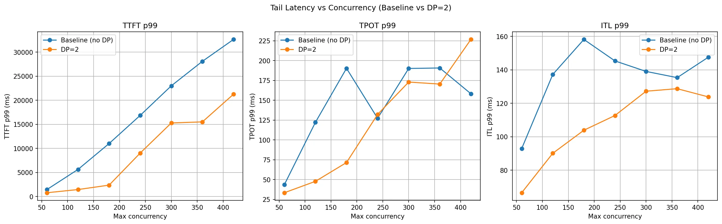
This is where DP makes its biggest impact. TTFT P99 (the wait time for the slowest 1% of requests) explodes for the baseline as concurrency climbs — at c=120 it's already at 5.6 seconds, and by c=420 it reaches over 32 seconds. DP=2 cuts this dramatically: at c=120 it's just 1.4 seconds, and at c=420 it stays under 22 seconds.

The intuition is simple: with only one GPU, requests queue up behind each other. The unlucky ones at the back of the queue wait through every request ahead of them. With two GPUs, the queue is roughly half the length on each rank, so tail latency improves substantially.

ITL P99 (inter-token latency) also improves with DP=2 across all concurrency levels, though the gains are smaller since ITL is more tied to per-token compute rather than queueing.

TPOT P99 tells a mixed story. DP=2 is better at low-to-medium concurrency but slightly worse at very high concurrency (c=420). At extreme load, the internal scheduler overhead and load imbalance between ranks can introduce some variability in how long individual decodes take.

What Is Pipeline Parallelism (PP)?

Pipeline Parallelism (PP) distributes model layers sequentially across GPUs, where GPU 0 processes layers 1-N, GPU 1 processes layers N+1-2N, and data flows through the pipeline.

Pipeline Parallelism splits the model by layers into stages. For example, early layers can be on GPU0 and later layers on GPU1. Unlike Tensor Parallelism (split inside a layer), PP splits across layers.

In PP inference, a request moves stage by stage: GPU0 computes its layers and sends the intermediate activations to GPU1, which computes the remaining layers and produces the output. Communication happens at stage boundaries, where activations are transferred between GPUs.

To use GPUs efficiently, systems often run multiple micro-batches in a pipeline. While one micro-batch is on stage 1 (GPU1), another can be on stage 0 (GPU0). This reduces idle time, but adds pipeline scheduling complexity.

PP is useful when a model is too large for one GPU but can fit when layers are distributed across GPUs. The trade-off is added latency from stage-to-stage activation transfers and possible pipeline bubbles when stages are unbalanced.

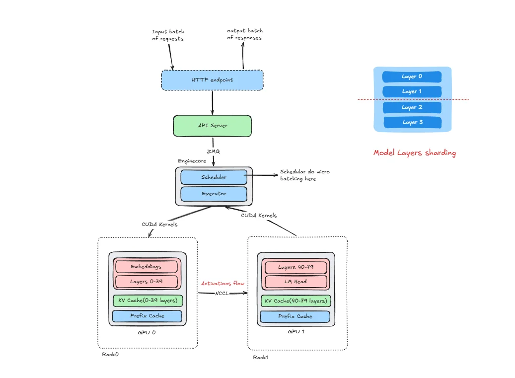
How vLLM Is Structured for PP

The components HTTP endpoint, API server, Engine Core, and ZMQ are the same as described in the DP section. What changes is how the model is partitioned and how ranks communicate internally.

In PP, each rank is a pipeline stage, not a full model replica. With PP=2 for a 80-layer model:

• Rank 0 runs on GPU 0 and holds the embedding layer plus layers 0–39 (the first half of the model).
• Rank 1 runs on GPU 1 and holds layers 40–79 (the second half of the model).

There is a single Engine Core (with its scheduler and executor) that manages both ranks together. Each rank has its own KV cache for its subset of layers and its own prefix cache. There is one API server shared across both ranks.

Communication channels:

• ZMQ: The API server talks to the Engine Core over ZMQ, the same as in DP.
• CUDA kernels: Engine core dispatches work to worker processes (IPC); workers then launch CUDA kernels on their GPUs.
• NCCL (send/recv): After Rank 0 finishes its forward pass through layers 0–39, it sends the resulting activation tensor to GPU 1 using NCCL point-to-point send/recv. This is the stage-boundary transfer. it happens every prefill step and every decode step.

This is the key structural difference from DP: in DP, ranks never talk to each other during inference. In PP, ranks are connected in a chain and must communicate at every forward pass.

---

Initialization

vllm serve Qwen/Qwen3-14B --pipeline-parallel-size 2

When this command runs, vLLM launches two rank processes (Rank 0 and Rank 1), each assigned to a GPU. The model is partitioned by layers:

• Rank 0 loads the embedding and the first 40 layers (0–39) into GPU 0 memory.
• Rank 1 loads the remaining 40 layers (40–79) into GPU 1 memory.

Each rank allocates its own KV cache for only its layers, and initializes a prefix cache. The NCCL communicator between GPU 0 and GPU 1 is initialized so that activation tensors can be transferred at stage boundaries. The single Engine Core starts its scheduler loop (which coordinates work across both ranks), and the API server begins listening. The system is now ready to serve.

---

Inference

Let's trace a single request through the pipeline.

Step 1: Request arrives — Client → HTTP endpoint → API server.

Step 2: The API server sends the request via ZMQ to the Engine Core.

Step 3: The Engine Core scheduler queues and batches the request, then the executor kicks off the prefill on Rank 0 (the first pipeline stage).

Step 4: Rank 0 forward pass — the embedding layer converts IDs to dense vectors, then layers 0–39 are computed on GPU 0. The KV cache for layers 0–39 is populated.

Step 5: Activation transfer — Rank 0 sends the output activation tensor from GPU 0 to GPU 1 via NCCL send/recv. This is a direct device-to-device transfer managed by NCCL, with no CPU involvement.

Step 6: Rank 1 forward pass — the activation arrives on GPU 1. Layers 40–79 are computed. The KV cache for layers 40–79 is populated.

Step 7: Rank 1 produces the output logits, samples the next token, and passes the result back through the pipeline.

Step 8: The token is sent back to the API server → streamed to the client.

For every subsequent decode step, steps 4–7 repeat. Each new token requires a full pipeline traversal: GPU 0 computes its layers using cached KV for layers 0–39, sends activations to GPU 1, GPU 1 computes with its cached KV for layers 40–79, and produces the next token. This sequential dependency is why PP increases per-token latency compared to a single-GPU setup.

---

KV Cache in Pipeline Parallelism

In PP, the KV cache is naturally distributed across stages:

• Rank 0 / GPU 0 (layers 0–39): Stores KV cache only for layers 0–39, plus a prefix cache for those layers.
• Rank 1 / GPU 1 (layers 40–79): Stores KV cache only for layers 40–79, plus a prefix cache for those layers.

This is different from TP where every GPU stores KV cache spanning all layers but only for its subset of attention heads. In PP, each GPU genuinely holds less KV cache because it only has a subset of layers.

Benefits:

• Memory per GPU is reduced proportionally to the number of stages
• No KV cache synchronization needed between stages

Drawbacks:

• For each generated token, the request must traverse all stages sequentially
• Rank 0 computes → sends activation → Rank 1 computes → final token
• This adds latency compared to TP where all GPUs work on the same token simultaneously

Implication for decode: During autoregressive decoding, every single token requires a full pipeline traversal. If you have 4 PP stages, each token generation has 4 sequential hops. With PP=2, there are 2 hops per token. This is why PP increases per-token latency even though it reduces memory per GPU.

What Are Pipeline Bubbles?

A pipeline bubble is a period where a GPU stage is idle — it has no work to do even though the system is actively processing requests. Bubbles are the core efficiency cost of pipeline parallelism and directly inflate ITL and TPOT. we have added Nsight screenshot for better understanding of this bubbles.

There are two distinct bubble patterns in a 2-stage pipeline:

Bubble type 1: GPU 0 idle while GPU 1 is busy

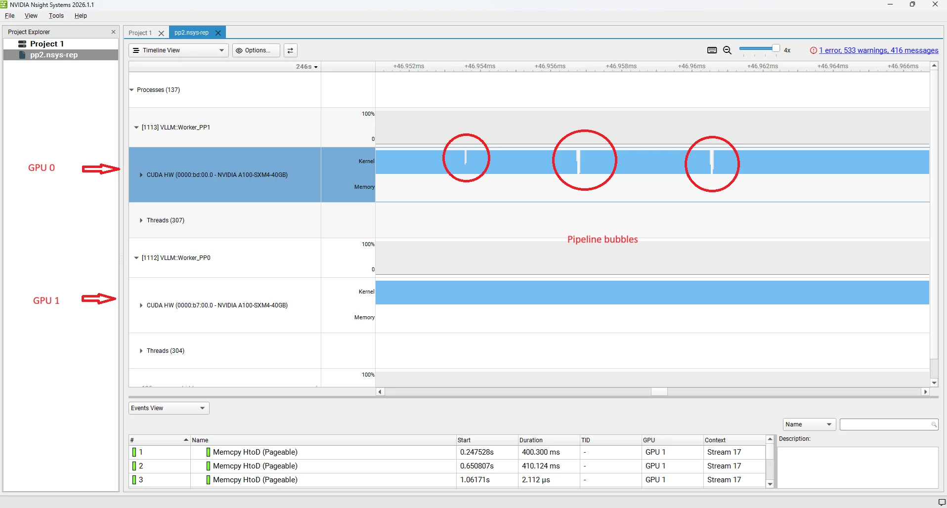
This happens when Rank 0 (GPU 0) finishes its layers and sends activations to Rank 1 (GPU 1), but Rank 1 takes longer than expected — for example, because it received a large batch, because it is handling a prefill-heavy step, or because it is generating logits and sampling. Rank 0 has already completed its portion and has nothing to start next until Rank 1 finishes and the scheduler releases the next batch to it. The gap on GPU 0 is backpressure from the downstream stage: the upstream stage is stalled because the downstream stage is the bottleneck.

Bubble type 2: GPU 1 idle while GPU 0 is busy

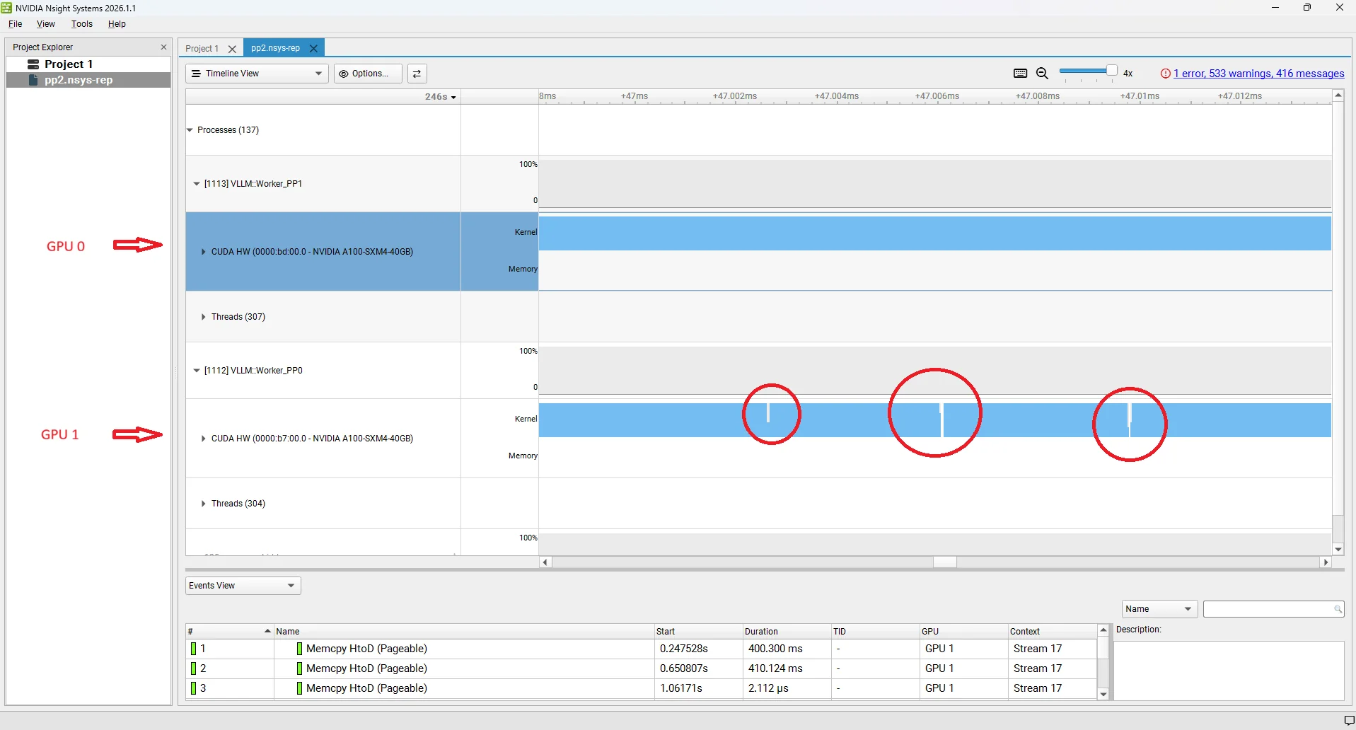
This is the opposite case. Rank 1 (GPU 1) has finished processing its batch and is waiting for the next activation tensor to arrive from Rank 0 (GPU 0). Rank 0 is still computing — because the batch is large, or because a long prefill arrived, or simply because layers 0–39 are computationally heavier for this particular sequence. Rank 1 has nothing to work on until the NCCL send/recv delivers the next activation. The gap on GPU 1 is a starvation bubble: the downstream stage is waiting for the upstream stage to produce work.

Both bubble types reduce effective GPU utilisation and translate directly into higher ITL at the system level: while one GPU is idle, no new tokens are being produced. In practice, the scheduler tries to keep the pipeline fed by overlapping decode batches from different requests — while GPU 1 handles one batch's forward pass, GPU 0 starts the next batch's layers. But perfect overlap is rarely achieved because decode step durations vary with sequence length, prefix cache hits, and batch composition. The residual idle time is what shows up as the bubble gaps in profiling traces and as elevated TPOT/ITL in benchmarks at high concurrency. Advanced techniques like virtual pipeline parallelism split stages into smaller chunks to reduce the bubble fraction.

Combining Pipeline and Tensor Parallelism for Large Models

In practice, PP and TP are often used together, especially for very large models across multiple nodes.

Common Configuration: TP within node, PP across nodes

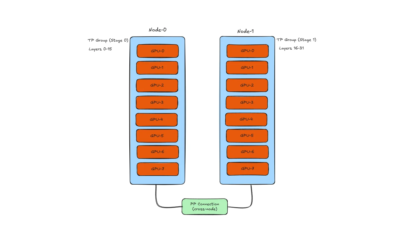
Why this layout?

• TP needs high bandwidth: All-reduce happens after every layer, so TP GPUs should be connected via NVLink (600+ GB/s)
• PP can tolerate lower bandwidth: Only activations transfer at stage boundaries, so slower cross-node links (100-400 Gb/s InfiniBand) are acceptable
• Result: Use fast intra-node links for TP, slower inter-node links for PP

Example with 16 GPUs (2 nodes × 8 GPUs):

Configuration	TP	PP	Description
TP=8, PP=2	8 GPUs per stage	2 stages	Each node is one PP stage, all 8 GPUs do TP within stage
TP=4, PP=4	4 GPUs per stage	4 stages	4 PP stages, each using 4-way TP
TP=2, PP=8	2 GPUs per stage	8 stages	More stages, less TP - higher latency but works with slower interconnect

vLLM usage:

vllm serve meta-llama/Llama-3-70B \
  --tensor-parallel-size 4 \
  --pipeline-parallel-size 2

This launches inference with 4-way TP and 2-way PP, requiring 8 GPUs total.

Trade-off summary:

• More TP → lower latency, but needs faster interconnect
• More PP → higher latency, but works with slower interconnect
• Balance based on your hardware topology

Note: We cover Tensor Parallelism in detail in the next section. Also, this blog focuses on single-node experiments only. Multi-node distributed inference (PP across nodes, cross-node TP) will be covered in a separate blog.

PP Benchmarks

Model: Qwen3-14B | GPUs: 2× A100-40GB | Dataset: ShareGPT | Strategy: Pipeline Parallelism

Experiment: Qwen/Qwen3-14B with ShareGPT dataset, comparing with and without PP, run on 2× NVIDIA A100 40GB GPUs.

The PP=2 server was profiled with NVIDIA Nsight Systems (nsys) to capture a detailed trace of GPU activity during inference:

# PP=2 (with nsys profiling — repeat with -o pp2_120, pp2_180 … for each concurrency level)
nsys profile -o pp2_60 \
  --trace-fork-before-exec=true \
  --trace=cuda,nvtx,osrt \
  --cuda-graph-trace=node \
  --delay=60 \
  vllm serve Qwen/Qwen3-14B \
    --pipeline-parallel-size 2 \
    --host 0.0.0.0 \
    --port 8000 \
    --dtype bfloat16 \
    --gpu-memory-utilization 0.92

**nsys profile parameters :**

Parameter	What it does
-o pp2_60	Output filename for the .nsys-rep profile trace. Change to pp2_120, pp2_180, etc. for each concurrency run so profiles don't overwrite each other.
--trace-fork-before-exec=true	Tells nsys to attach to child processes that are forked before exec(). This is essential for vLLM, which spawns separate rank worker processes at startup — without this flag only the parent process is traced and all GPU activity on the worker ranks is invisible.
--trace=cuda,nvtx,osrt	Captures three event streams: CUDA API calls and GPU kernel timings (cuda), manual annotation markers placed by vLLM to label regions like prefill and decode (nvtx), and OS-level runtime events such as thread creation and mutex waits (osrt). Together these give a complete picture of where time is spent during inference.
--cuda-graph-trace=node	When vLLM replays a CUDA graph, this flag breaks the trace down to individual operation nodes inside the graph instead of showing the entire replay as a single opaque block. Without it, CUDA graph regions appear as one undifferentiated entry and per-kernel timing is lost.
--delay=60	Waits 60 seconds before the profiler starts recording. This skips model loading, weight sharding across ranks, KV cache allocation, and NCCL communicator initialization. The trace then captures only steady-state serving traffic, which is what matters for inference analysis.

# Baseline (no PP)
vllm serve Qwen/Qwen3-14B \
  --dtype bfloat16 \
  --host 0.0.0.0 \
  --gpu-memory-utilization 0.92 \
  --max-model-len 20480 \
  --port 8000

Each data point comes from a separate client run, varying only --max-concurrency. First, download the ShareGPT dataset using command given in DP section.

Then run the benchmark:

vllm bench serve \
  --model Qwen/Qwen3-14B \
  --dataset-name sharegpt \
  --dataset-path ./ShareGPT_V3_unfiltered_cleaned_split.json \
  --host 127.0.0.1 \
  --port 8000 \
  --max-concurrency 60 \
  --seed 42 \
  --num-prompts 1000

Everything else stays fixed — same model, same dataset, same 1,000 prompts, same random seed. The only knob being turned is --max-concurrency. This gives a clean comparison of how each configuration behaves under increasing load.

The key pattern to watch: PP=2 won't double throughput (it's not adding a second replica), but it should reduce TTFT significantly at high concurrency by giving both GPUs more KV cache headroom.

Metric	Config	c=60	c=120	c=180	c=240	c=300	c=360	c=420
Output Throughput (tok/s)	Baseline (no PP)	1,333.94	1,589.01	1,551.60	1,557.29	1,679.27	1,600.59	1,560.00
	PP=2	1,391.51	1,579.03	1,545.54	1,658.22	1,561.35	2,240.86	2,030.76
Total Throughput (tok/s)	Baseline (no PP)	2,768.04	3,293.47	3,218.96	3,236.12	3,495.46	3,326.92	3,242.04
	PP=2	2,884.05	3,286.78	3,208.54	3,441.06	3,242.76	4,666.63	4,208.26
TTFT P99 (ms)	Baseline (no PP)	1,917.43	3,331.34	8,682.55	15,618.11	21,744.46	28,996.97	34,182.93
	PP=2	1,764.29	2,395.14	3,043.66	3,965.23	6,340.30	8,966.51	13,093.53
TPOT P99 (ms)	Baseline (no PP)	66.44	146.12	253.09	263.42	261.90	263.54	262.16
	PP=2	52.81	97.14	176.10	245.41	165.65	232.26	239.47
ITL P99 (ms)	Baseline (no PP)	114.54	180.70	252.47	261.80	264.05	264.18	264.64
	PP=2	113.77	175.14	229.76	257.76	273.40	242.79	219.07

Throughput comparison

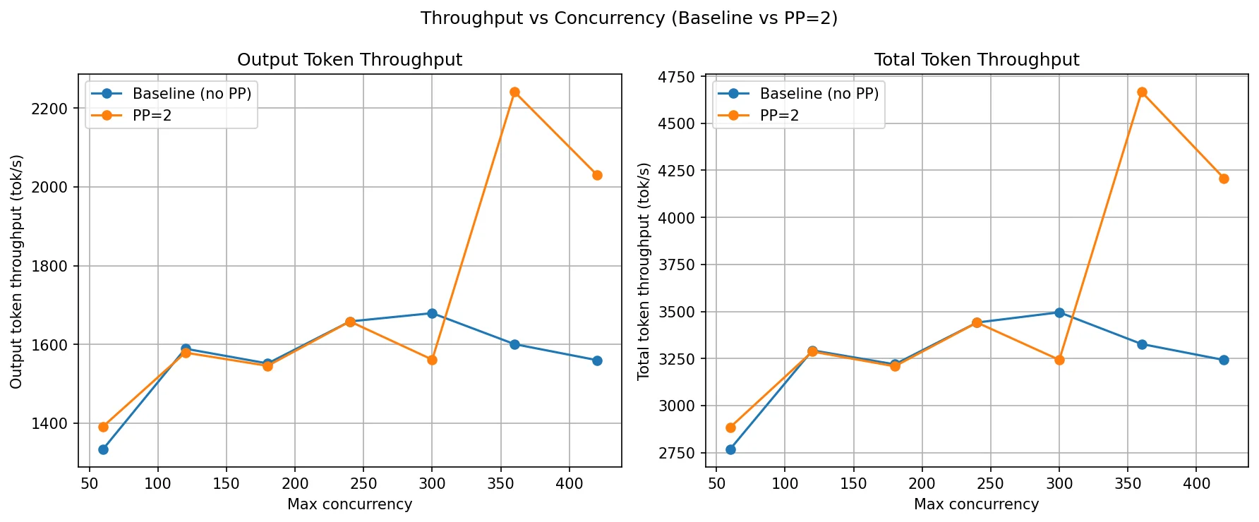
PP=2 throughput closely tracks the baseline at low-to-medium concurrency (c=60 to c=240). Both curves plateau around 1,550–1,680 tok/s by c=120 — the single-pipeline compute capacity is saturated. Unlike DP, PP=2 does not add a second independent replica, so there is no doubling of throughput. The model is still processed sequentially one stage at a time.

The interesting shift happens at c=360 and c=420, where PP=2 jumps to 2,240 and 2,030 tok/s while the baseline actually dips back to 1,600 and 1,560. This is a KV cache effect: by splitting layers across two GPUs, each GPU's memory holds only half the model weights. That frees up more GPU memory on each rank for KV cache. At very high concurrency, the baseline's single GPU is KV-cache-constrained and starts evicting or throttling requests, capping throughput. PP=2's larger total KV cache allows it to keep more requests in-flight and form bigger decode batches, which is why throughput rises at the high end.

TTFT, TPOT and ITL comparison

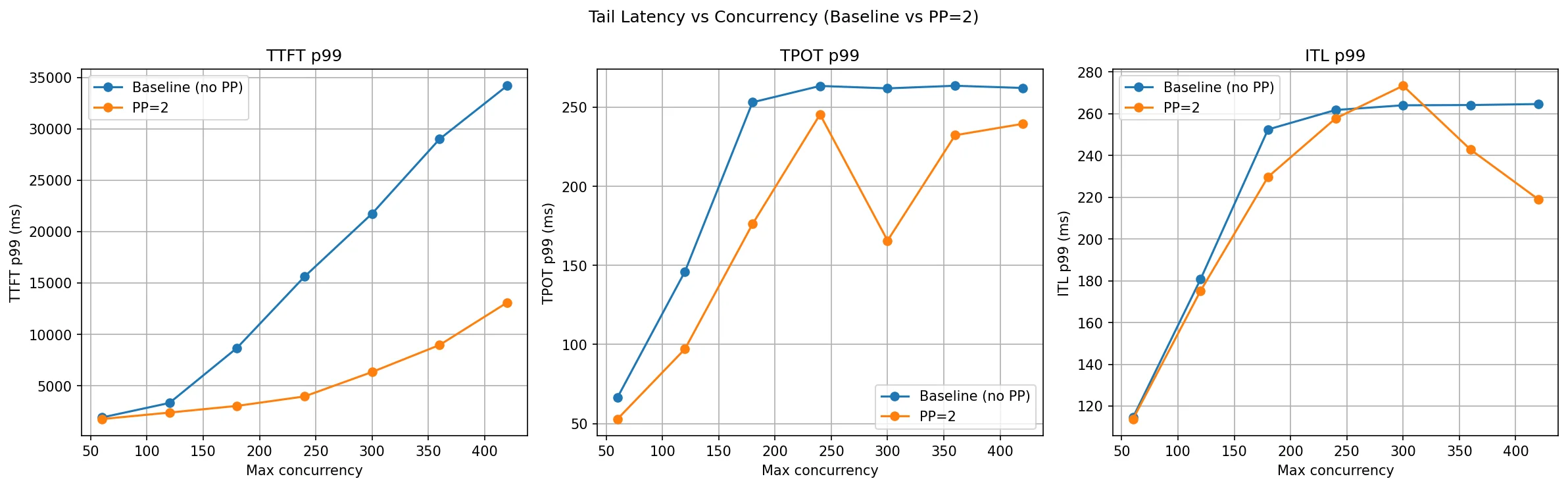
This is where PP=2 shows its clearest win. TTFT P99 for the baseline explodes as concurrency grows — at c=180 it is already at 8.6 seconds and by c=420 it reaches 34 seconds. PP=2 holds TTFT P99 to 3 seconds at c=180 and just 13 seconds at c=420, roughly a 2.5–3× improvement throughout the high-concurrency range.

The mechanism is again KV cache capacity. With one GPU, once the KV cache fills up, new requests are queued and wait longer and longer for their prefill to run — that wait is what TTFT measures. PP=2's larger aggregate KV cache delays the point at which the system starts queuing, so the tail of the TTFT distribution stays controlled for longer.

TPOT P99 also improves with PP=2 at most concurrency levels. At c=60 it drops from 66 ms to 52 ms, and at c=300 from 262 ms to 165 ms. The extra KV cache headroom allows the scheduler to form larger and more consistent decode batches, smoothing out per-token latency spikes.

ITL P99 tells a mixed story — PP=2 is better through c=240 but slightly worse at c=300 (273 ms vs 264 ms), after which it recovers. At the very point where the baseline's KV cache is most constrained, the scheduler on both configs starts making suboptimal batching decisions, and the pipeline latency overhead of NCCL transfers between Rank 0 and Rank 1 adds a small but visible floor to ITL that the baseline (single GPU) doesn't have.

What Is Tensor Parallelism (TP)?

Tensor Parallelism (TP) splits each transformer layer's weight matrices across multiple GPUs, with all GPUs computing in parallel and synchronizing via NCCL all-reduce after each layer.

Tensor Parallelism splits the heavy math inside each layer across multiple GPUs rather than splitting the model by layers (as PP does). Every GPU runs every layer, but each GPU owns only a shard of the weight matrices. After computing their partial results the GPUs synchronize via NCCL collective operations to produce the correct full output before moving to the next layer.

The key structural difference from PP is visible in the following diagram: both ranks hold shards of all layers (not a subset), and the 2-way NCCL arrows run between ranks at every single layer boundary. After the final layer, each rank computes partial logits from its LM head shard. An NCCL all-gather assembles the full logits on every rank, and all ranks independently sample the same next token (using deterministic sampling with synchronized seeds — no broadcast needed).

The key idea: layers are not split by depth but by width. Both GPUs collaborate on every forward pass for every request in lockstep, leveraging GPU parallel computing capabilities — there is no sequential stage dependency as in PP.

Here :

• HTTP Endpoint and API Server : same single entry point as in DP and PP.
• Engine Core : one Engine Core manages both ranks, connected to the API server over ZMQ.
• Rank 0 (GPU 0) and Rank 1 (GPU 1) : each rank holds a shard of every layer's weight matrices (not a subset of layers as in PP). Both ranks hold the full model depth but only half the width of each weight tensor.
• 2-way NCCL arrows between ranks : after each layer's partial compute, both ranks perform an NCCL collective (all-reduce for MLP, all-reduce / all-gather for attention) to combine their partial results. This happens at every single layer boundary.
• Logits all-gather : after the final layer, each rank computes partial logits from its LM head shard. An NCCL all-gather assembles the full logits on every rank. All ranks then independently sample the same next token using deterministic sampling with synchronized seeds.
• ZMQ : the API server communicates with the Engine Core over ZMQ, identical to DP and PP.

In the following sections we will see how this actually works for MLP and attention layers. Note that LayerNorm, Dropout, and Residual connections are not sharded. they are cheap and are replicated identically on each GPU.

Tensor Parallelism in Multi Layer Perceptron

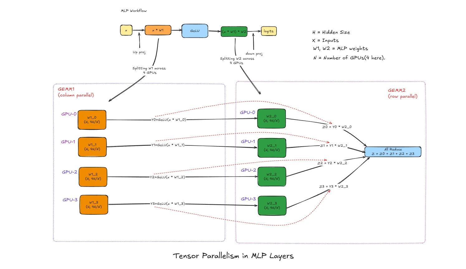
x : Input activation vector (after LayerNorm), shape [batch, H]

H: Hidden size (embedding dimension) of the model

N : Number of GPUs used for tensor parallelism (4 in this diagram)

W1 : First MLP weight matrix, shape [H, 4H] (expands hidden dim)

W2 : Second MLP weight matrix, shape [4H, H] (projects back down)

W1_i : Column shard of W1 on GPU i, shape [H, 4H/N]

W2_i : Row shard of W2 on GPU i, shape [4H/N, H]

Y_i : Intermediate output on GPU i after GEMM1 + GeLU

Z_i : Partial output on GPU i after GEMM2

Z : Final MLP output after all-reduce, shape [batch, H]

What is GEMM?

GEMM stands for General Matrix Multiply. It's just matrix multiplication - taking two matrices and multiplying them together.

In simple terms:

• You have a matrix A (your input data)
• You have a matrix B (your weights)
• GEMM computes: Output = A × B

Why the fancy name? Because GPUs have specialized hardware (tensor cores) optimized specifically for this operation. When we say "GEMM1" and "GEMM2" in the MLP, we're just referring to the first and second matrix multiply operations in that layer.

Think of it like this: if your input x has shape [batch, 4096] and weight W1 has shape [4096, 16384], the GEMM produces output shape [batch, 16384]. Each output element is computed by multiplying a row from x with a column from W1 and summing the results.

Normal MLP Workflow (Without Parallelism)

The standard MLP block in a transformer follows this flow:

x → GEMM1 (x × W1) → GeLU → GEMM2 (result × W2) → output

• GEMM1: Expands the hidden dimension from H to 4H
• GeLU: Element-wise non-linear activation
• GEMM2: Projects back from 4H to H

This block is extremely compute-heavy and memory-heavy. For large models like Llama-70B, W1 and W2 together can be several gigabytes per layer. Running this on a single GPU becomes a memory bottleneck, which is why tensor parallelism splits this work.

Tensor Parallelism Step-by-Step

GEMM1 with Column Parallelism

The weight matrix W1 of shape [H, 4H] is split column-wise across N GPUs:

W1 = [W1_0 | W1_1 | W1_2 | W1_3]
      ↓      ↓      ↓      ↓
     GPU0   GPU1   GPU2   GPU3

Each W1_i has shape [H, 4H/N].

All GPUs receive the same input x. Each GPU computes only its portion:

• GPU0: x × W1_0 → result shape [batch, 4H/N]
• GPU1: x × W1_1 → result shape [batch, 4H/N]
• GPU2: x × W1_2 → result shape [batch, 4H/N]
• GPU3: x × W1_3 → result shape [batch, 4H/N]

No communication needed after GEMM1 because each GPU has an independent chunk of the expanded representation.

GeLU Activation (Local)

Each GPU applies GeLU to its local GEMM1 output:

• GPU0: Y0 = GeLU(x × W1_0)
• GPU1: Y1 = GeLU(x × W1_1)
• GPU2: Y2 = GeLU(x × W1_2)
• GPU3: Y3 = GeLU(x × W1_3)

GeLU is element-wise, so it operates independently on each shard. No communication needed.

GEMM2 with Row Parallelism

The weight matrix W2 of shape [4H, H] is split row-wise across N GPUs:

W2 = [ W2_0 ]    ← GPU0 owns this row block
     [ W2_1 ]    ← GPU1 owns this row block
     [ W2_2 ]    ← GPU2 owns this row block
     [ W2_3 ]    ← GPU3 owns this row block

Each W2_i has shape [4H/N, H].

Each GPU multiplies its local Y_i with its local W2_i:

• GPU0: Z0 = Y0 × W2_0 → shape [batch, H]
• GPU1: Z1 = Y1 × W2_1 → shape [batch, H]
• GPU2: Z2 = Y2 × W2_2 → shape [batch, H]
• GPU3: Z3 = Y3 × W2_3 → shape [batch, H]

Each Z_i is a partial contribution to the final output, not the complete result.

All-Reduce to Combine Results

The final output requires summing all partial results:

Z = Z0 + Z1 + Z2 + Z3

This is done via all-reduce sum collective operation. After all-reduce:

• Every GPU has the identical final output Z
• The result is mathematically equivalent to GeLU(x × W1) × W2 computed on a single GPU
• The model can proceed to the next layer (attention or another MLP block)

Why This Split Works Mathematically

The column-row split is chosen specifically so that only one communication point (after GEMM2) is needed per MLP block.

If we write the full MLP as:

output = GeLU(x × W1) × W2

With column split of W1 and row split of W2:

output = GeLU(x × [W1_0|W1_1|W1_2|W1_3]) × [W2_0; W2_1; W2_2; W2_3]
       = [GeLU(x×W1_0) | GeLU(x×W1_1) | GeLU(x×W1_2) | GeLU(x×W1_3)] × [W2_0; W2_1; W2_2; W2_3]
       = GeLU(x×W1_0)×W2_0 + GeLU(x×W1_1)×W2_1 + GeLU(x×W1_2)×W2_2 + GeLU(x×W1_3)×W2_3
       = Z0 + Z1 + Z2 + Z3

This is exactly what the all-reduce sum computes.

---

Tensor Parallelism in Attention Layers

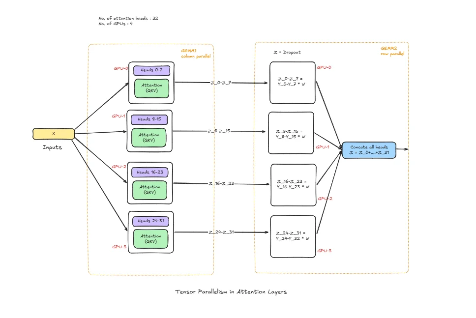
num_heads : Total attention heads

head_dim : Per-head dimension (H = num_heads * head_dim)

Wq, Wk, Wv : Query, Key, Value projection weights

Wo : Output projection weight

Wq_i, Wk_i, Wv_i : Local Q/K/V shards on GPU i

Wo_i : Local output-projection shard on GPU i

Q_i, K_i, V_i : Local projected tensors on GPU i

O_i : Local attention output contribution on GPU i

O : Final attention output after collective communication

Normal Attention Workflow (Without Parallelism)

In a standard transformer layer, attention follows this flow:

x -> Q,K,V projection -> score = QK^T / sqrt(head_dim) -> softmax(score) -> softmax(score) * V -> output projection (Wo) -> output

This block is expensive because projection and attention math scale with sequence length and hidden size. On larger models and longer contexts, memory and compute pressure becomes very high on a single GPU.

Tensor Parallelism Step-by-Step

QKV Projection Split (Head/Channel Parallelism)

Q/K/V projection weights are split across GPUs by head/channels. Each GPU receives the same input x, but multiplies only with its local weight shards:

• GPU0 computes Q0, K0, V0
• GPU1 computes Q1, K1, V1
• GPU2 computes Q2, K2, V2
• GPU3 computes Q3, K3, V3

Each GPU now owns only its subset of heads.

Local Attention Compute

Each GPU performs attention on its local heads:

• Compute scores: S_i = Q_i K_i^T / sqrt(head_dim)
• Apply softmax on S_i
• Multiply by local V_i to get local context

This is the most compute-heavy part and stays local, which is why TP helps.

Output Projection (Wo)

After local context is formed, output projection is applied with sharded Wo. Each GPU produces a partial output contribution O_i. This is not yet the full hidden output.

Collective Communication (All-Reduce / All-Gather)

At the boundary, GPUs communicate to build the final output O. Depending on implementation layout, this is typically all-reduce sum or all-gather + combine.

After this step:

• Every GPU has the correct full attention output for the next layer
• Result is mathematically equivalent to single-GPU attention, but memory and compute are distributed

Why This Split Is Used

Attention TP is designed to keep the heavy work (QKV projection and per-head attention math) local on each GPU, and introduce communication only when full hidden representation is needed. This reduces per-GPU memory load and enables larger models to run efficiently across multiple GPUs.

---

Why GEMM vs GEMV Matters for LLM Inference

• GEMM dominates when batch/tokens processed together are larger
• GEMV appears in low-batch or token-by-token decode behavior
• TP helps both, but comm overhead is more visible when compute per step is small (GEMV-heavy decode)

So in benchmarks:

• At low concurrency, TP may not always win TTFT
• At higher concurrency/throughput-focused runs, TP usually shows stronger Tok/s scaling

---

How vLLM Is Structured for TP

The components HTTP endpoint, API server, Engine Core, and ZMQ are the same as described above. What changes is how the model is held and how ranks communicate during inference.

With TP=2 for a 80-layer model:

• Rank 0 runs on GPU 0 and holds shards of all 80 layers. specifically half the columns of every Q/K/V/O weight matrix in attention and half the columns of W1 / half the rows of W2 in every MLP block.
• Rank 1 runs on GPU 1 and holds the complementary shards of the same 80 layers.

Both ranks hold a shard of the embedding layer (partitioned along the vocabulary dimension). After embedding lookup, an all-reduce produces the identical hidden state on both ranks. There is a single Engine Core (with scheduler and executor) that drives both ranks in lockstep. Each rank stores a KV cache only for the attention heads it owns — with TP=2, each GPU gets total_heads / 2 heads. This KV cache spans all 80 layers (because both ranks participate in every layer), but only for that rank's half of the heads. Rank 0 stores keys and values for its head subset across all layers; Rank 1 stores the complementary head subset across all layers.

Communication channels:

• ZMQ: The API server talks to the Engine Core over ZMQ, unchanged from DP/PP.
• CUDA kernels: Used for communication between the Engine Core and rank workers.
• NCCL all-reduce / all-gather: After every MLP block and every attention block, the two ranks perform an NCCL collective to combine partial results. This is the dominant inter-GPU communication pattern — it happens at each of the 80 layers for every forward pass.
• NCCL all-gather (logits): After the final layer, each rank computes partial logits from its LM head shard. An NCCL all-gather assembles the full logits on every rank. All ranks then independently sample the same next token using deterministic sampling with synchronized seeds — no token broadcast is needed.

This is the key structural difference from both DP and PP: in TP, both ranks must synchronize at every layer boundary of every forward pass. The all-reduce frequency is much higher than PP's single stage-boundary transfer, which is why TP requires fast interconnects (NVLink ideally) to avoid the per-layer communication becoming the bottleneck.

---

Initialization

vllm serve Qwen/Qwen3-14B --tensor-parallel-size 2

When this command runs, vLLM launches two rank processes (Rank 0 and Rank 1), each assigned to a GPU. The model weights are loaded and sharded:

• For every attention layer: Q/K/V/O weight matrices are split column-wise across the two ranks by attention head.
• For every MLP block: W1 is split column-wise, W2 is split row-wise.
• LayerNorm and residual connections are replicated on both GPUs. Embeddings are sharded along the vocabulary dimension.

Each rank allocates a KV cache that covers all 80 layers but only for its owned attention heads (total_heads / 2 heads per rank). This is less KV cache per GPU than the single-GPU baseline — the total across both ranks equals one full model's KV cache, just split by head ownership. The NCCL communicator group is initialized between GPU 0 and GPU 1 — this sets up the all-reduce and broadcast channels used during inference. The single Engine Core starts its scheduler loop, and the API server begins listening. The system is now ready to serve.

---

Inference

Let's trace a single request through the TP=2 system.

Step 1: Request arrives — Client → HTTP endpoint → API server.

Step 2: The API server sends the request via ZMQ to the Engine Core.

Step 3: The Engine Core scheduler queues and batches the request, then the executor dispatches the prefill to both ranks simultaneously.

Step 4: Both ranks receive the same tokenized input. Each rank looks up tokens in its local embedding shard. An all-reduce combines the partial results so both ranks start with the identical initial hidden state.

Step 5: For each of the 80 layers, both ranks run in lockstep:

• Attention: Each rank computes Q/K/V projections for its head shard, runs attention locally, applies its shard of Wo. An NCCL all-reduce sums the partial outputs so both ranks hold the identical attention output.
• MLP: Each rank computes GEMM1 (column shard) + GeLU locally, then GEMM2 (row shard). An NCCL all-reduce sums the partial results so both ranks hold the identical MLP output.
• LayerNorm and residual are applied locally (identical on both ranks since their inputs are identical after each all-reduce).

Step 6: After the final layer, both ranks hold the same final hidden state. Each rank computes partial logits from its LM head shard. An NCCL all-gather assembles the full logits on every rank, and all ranks independently sample the same next token (deterministic sampling with synchronized seeds).

Step 7: The token is returned to the Engine Core → API server → streamed to the client.

For every subsequent decode step, steps 5–7 repeat. Each new token triggers a full lockstep pass through all 80 layers on both GPUs, with two NCCL all-reduces per layer (one for attention, one for MLP). This is why TP reduces per-token latency: both GPUs are computing in parallel throughout the entire forward pass, not sequentially as in PP.

---

TP Benchmarks

Model: Qwen3-14B | GPUs: 2× A100-40GB | Dataset: ShareGPT | Strategy: Tensor Parallelism

Experiment: Qwen/Qwen3-14B with ShareGPT dataset, comparing with and without TP, run on 2× NVIDIA A100 40GB GPUs.

The TP=2 server was profiled with NVIDIA Nsight Systems:

# TP=2 (with nsys profiling — repeat with -o tp_120, tp_180 … for each concurrency level)
nsys profile -o tp_60 \
  --trace-fork-before-exec=true \
  --trace=cuda,nvtx,osrt \
  --cuda-graph-trace=node \
  --delay=60 \
  vllm serve Qwen/Qwen3-14B \
    --tensor-parallel-size 2 \
    --host 0.0.0.0 \
    --port 8000

The nsys profile parameters are the same as described in the PP benchmarks section above: --trace-fork-before-exec=true captures all rank worker processes, --trace=cuda,nvtx,osrt records GPU kernels, vLLM annotations, and OS thread events, --cuda-graph-trace=node exposes per-kernel timing inside CUDA graph replays, and --delay=60 skips model loading so only steady-state inference is traced.

Note (profiling vs. measurement): The nsys profile command above is used solely to capture Nsight traces for the kernel-level visualisations. All benchmark numbers in the tables below come from separate runs without nsys profile — profiling adds overhead that would distort throughput and latency measurements.

# Baseline (no TP)
vllm serve Qwen/Qwen3-14B \
  --dtype bfloat16 \
  --host 0.0.0.0 \
  --gpu-memory-utilization 0.95 \
  --max-model-len 20480 \
  --port 8000

Each data point comes from a separate client run, varying only --max-concurrency. First, download the ShareGPT dataset:

wget https://huggingface.co/datasets/anon8231489123/ShareGPT_Vicuna_unfiltered/resolve/main/ShareGPT_V3_unfiltered_cleaned_split.json

Then run the benchmark:

vllm bench serve \
  --model Qwen/Qwen3-14B \
  --dataset-name sharegpt \
  --dataset-path ./ShareGPT_V3_unfiltered_cleaned_split.json \
  --host 127.0.0.1 \
  --port 8000 \
  --max-concurrency 60 \
  --seed 42 \
  --num-prompts 1000

Everything else stays fixed — same model, same dataset, same 1,000 prompts, same random seed. The only knob being turned is --max-concurrency. This gives a clean comparison of how each configuration behaves under increasing load.

Note (stress-test mode): --request-rate is not set and defaults to inf, meaning all 1,000 prompts are submitted simultaneously. This is a deliberate stress-test that maximises concurrency pressure to reveal peak throughput and tail-latency ceilings. It does not model a realistic Poisson arrival process.

In the following table each column (c=60 to c=420) is a separate benchmark run with that many concurrent requests. Higher is better for throughput, lower is better for latency. The key pattern to watch: unlike PP, TP=2 should show a clear throughput lift even at low concurrency because both GPUs contribute to every single request in parallel.

Metric	Config	c=60	c=120	c=180	c=240	c=300	c=360	c=420
Output Throughput (tok/s)	Baseline (no TP)	1,333.94	1,589.01	1,551.60	1,557.29	1,679.27	1,600.59	1,560.00
	TP=2	2,225.31	2,774.31	2,605.26	2,843.41	2,676.99	2,676.27	2,679.59
Total Throughput (tok/s)	Baseline (no TP)	2,768.04	3,293.47	3,218.96	3,236.12	3,495.46	3,326.92	3,242.04
	TP=2	4,622.94	5,768.36	5,403.84	5,914.84	5,562.16	5,548.66	5,555.37
TTFT P99 (ms)	Baseline (no TP)	1,917.43	3,331.34	8,682.55	15,618.11	21,744.46	28,996.97	34,182.93
	TP=2	1,160.32	2,027.32	2,954.72	3,984.22	5,129.20	7,876.75	11,587.95
TPOT P99 (ms)	Baseline (no TP)	66.44	146.12	253.09	263.42	261.90	263.54	262.16
	TP=2	42.15	84.49	147.64	157.51	159.79	158.87	161.59
ITL P99 (ms)	Baseline (no TP)	114.54	180.70	252.47	261.80	264.05	264.18	264.64
	TP=2	75.33	111.26	147.86	164.63	163.08	165.22	166.81

Throughput comparison

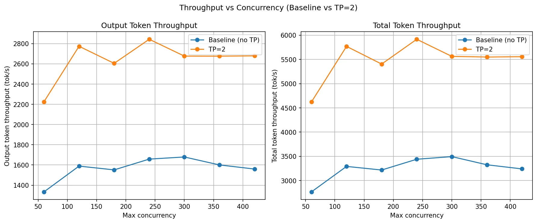
TP=2 delivers a consistent and substantial throughput gain across the entire concurrency range. At c=60, output throughput jumps from 1,334 tok/s to 2,225 tok/s — a ~67% increase even before queueing pressure builds up. This is the defining characteristic of TP: because both GPUs execute every layer together, each forward pass completes faster. The benefit is immediate, not just at high load.

The baseline plateaus around 1,550–1,680 tok/s from c=120 onward — a single GPU is saturated. TP=2 continues scaling, peaking at 2,774 tok/s at c=120 and stabilising around 2,600–2,840 tok/s across c=180 to c=420. Total throughput tracks the same pattern, staying near 5,400–5,900 tok/s for TP=2 at all concurrency levels above c=120, compared to 3,200–3,500 tok/s for the baseline.

The plateau in TP=2 throughput above c=120 is expected: both GPUs are now compute-saturated together. Adding more concurrency beyond that point just fills the scheduler queue rather than producing more tokens per second. Importantly, TP=2's plateau sits roughly 65–70% higher than the baseline's plateau — the gain is held steadily because the NCCL all-reduce overhead per layer is small relative to the compute savings from splitting the matrix multiplications.

TTFT, TPOT and ITL comparison

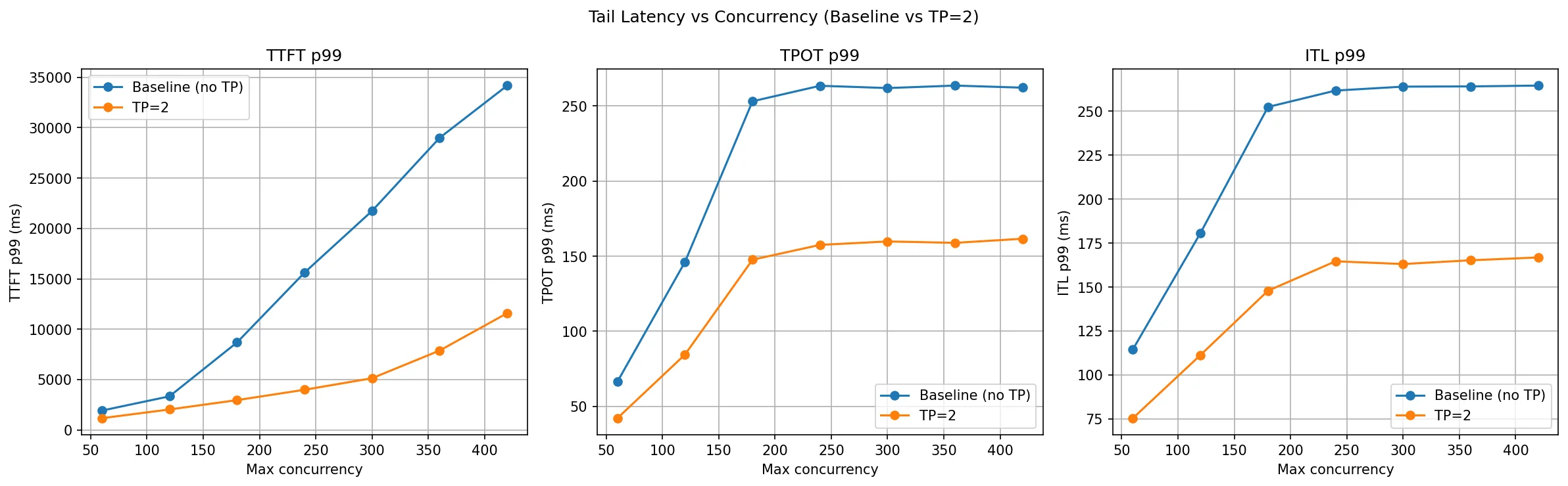
TP=2 wins clearly on all three latency metrics, and unlike PP the gains hold uniformly across all concurrency levels without the mixed signals seen in ITL.

TTFT P99 is dramatically reduced. At c=180 the baseline is already at 8.6 seconds; TP=2 keeps it to 2.9 seconds. By c=420, the baseline hits 34 seconds while TP=2 stays at 11.6 seconds — a 3× improvement at the tail. The reason is straightforward: with two GPUs splitting every matrix multiply, prefill computation finishes faster. A prompt that would take one GPU 100 ms to prefill takes TP=2 roughly 50–60 ms (not perfectly half, due to NCCL all-reduce overhead). At high concurrency, many requests are waiting for prefill, so faster per-prefill compute feeds requests through the queue faster.

TPOT P99 improves consistently across every concurrency level. At c=60 it drops from 66 ms to 42 ms; at c=300–c=420 it stabilises around 159–162 ms versus the baseline's 262–263 ms. This is a direct consequence of faster matrix multiplications per decode step each token generation involves fewer GPU milliseconds on each individual GPU, and the all-reduce cost (which is much cheaper than the compute it replaces) doesn't undo the gain.

ITL P99 is the cleanest story across all three strategies. TP=2 improves ITL at every concurrency level without exception: from 75 ms vs. 114 ms at c=60 to 166 ms vs. 264 ms at c=420. Because TP reduces actual compute time per token (not just queueing effects), the inter-token cadence is more consistent. There are no crossover points or mixed results as seen with PP. This consistency makes TP the better choice when token streaming latency matters.

---

DP vs PP vs TP: Which Parallelism Strategy Should You Use?

Based on the benchmarks across DP, PP, and TP on Qwen3-14B and Qwen3-32B with the ShareGPT dataset, here is a clear summary of what each strategy actually delivers.

Data Parallelism vs Pipeline Parallelism vs Tensor Parallelism

Strategy	Best For	Latency Impact	Throughput Impact	Memory per GPU	Communication	GPU Interconnect Requirement
DP	High throughput	No improvement	Linear scaling	Full model per GPU	None between replicas	None
PP	Memory-constrained	Higher (pipeline bubbles)	Moderate	Reduced (layer split)	Activation passing	Moderate (PCIe sufficient)
TP	Low latency	Significant reduction	Moderate	Reduced (tensor split)	All-reduce per layer	High (NVLink recommended)
DP + TP	Throughput + latency	Reduced per replica	Near-linear	Reduced per replica	All-reduce within TP group	NVLink within TP group

Benchmark Results Summary

Strategy	Throughput gain	TTFT improvement	ITL improvement	Requirement
DP=2	~50% at c=120–180, inconsistent at high load	2× at c=120, degrades less than baseline	Consistent improvement at all levels	Model must fit on a single GPU
PP=2	Minimal until very high concurrency (c=360+)	2.5–3× at c=180–420	Mixed better up to c=240, noisy beyond	Works with any interconnect speed
TP=2	~67% gain from c=60 onward, stable plateau	3× at c=180–420	Clean improvement at every level	Requires fast interconnect (NVLink)

How to Choose tensor-parallel-size and pipeline-parallel-size in vLLM

# Data Parallelism: replicate the model across GPUs for higher throughput
vllm serve <model> --data-parallel-size N

# Pipeline Parallelism: split model layers across GPUs for memory scaling
vllm serve <model> --pipeline-parallel-size N

# Tensor Parallelism: shard each layer across GPUs for lower latency
vllm serve <model> --tensor-parallel-size N

# Combined: TP within node, PP across nodes (total GPUs = N × M)
vllm serve <model> --tensor-parallel-size N --pipeline-parallel-size M

Use DP when your model fits on a single GPU and you need more throughput. DP is the simplest strategy with the most predictable results. It scales request-handling capacity by adding replicas, keeps latency low because each rank runs fully independently, and requires no inter-GPU communication during inference. The only real constraint is that the model must fit comfortably on one GPU including the KV cache.

Use PP when the model is too large for a single GPU and you do not have NVLink-class interconnects. PP distributes the model by layers so each GPU only needs to hold a fraction of the weights. Its TTFT win at high concurrency comes from a larger aggregate KV cache, not from faster compute. Per-token latency is higher than a single GPU because every decode step requires a full pipeline traversal through all ranks. If your primary constraint is memory and not latency, PP is the right tool.

Use TP when you need the lowest possible latency and have GPUs connected with NVLink or a similarly fast fabric. TP reduces actual compute time per forward pass by splitting the matrix math across GPUs. It wins on throughput, TTFT, TPOT, and ITL simultaneously and unlike PP it does so consistently across all concurrency levels, not just at the high end. The cost is that it requires frequent NCCL all-reduce calls at every layer boundary on a slow interconnect this communication overhead can wipe out the compute savings.

The key mental model: If you are limited by request volume, use DP. If you are limited by GPU memory, use PP. If you are limited by compute speed and latency, use TP.

In practice, these strategies are combined:

• For a single node with NVLink: prefer TP. Add DP on top if you have spare capacity.
• For multi-node or slow cross-node links: use TP within each node, PP across nodes.
• When model fits on one GPU: DP is the default first choice.

---

Frequently Asked Questions

What is the difference between tensor parallelism and pipeline parallelism?

Tensor parallelism splits each layer's matrix math across GPUs — all GPUs work on the same request simultaneously and synchronize via all-reduce after each layer. Pipeline parallelism splits the model by layers — GPU 0 runs early layers, GPU 1 runs later layers, and data flows sequentially through the pipeline. TP gives lower latency but needs fast interconnects (NVLink); PP works with slower links but adds per-token latency from pipeline traversal.

How many GPUs do I need for tensor parallelism in vLLM?

Set --tensor-parallel-size to the number of GPUs. For a 70B model in FP16 (~140GB), you need at least 2× A100-80GB GPUs with TP=2. For best performance, use GPUs connected via NVLink. The total GPU count equals tensor-parallel-size × pipeline-parallel-size × data-parallel-size.

Can I combine tensor parallelism and pipeline parallelism in vLLM?

Yes. Use --tensor-parallel-size N --pipeline-parallel-size M. The total GPUs needed is N × M. A common setup for multi-node is TP within a node (for fast NVLink communication) and PP across nodes. You can also add --data-parallel-size on top for additional throughput.

When should I use pipeline parallelism instead of tensor parallelism?

Use PP when your GPUs don't have fast interconnects (e.g., PCIe instead of NVLink), or when you need to fit a model across nodes. PP has lower communication overhead than TP but introduces pipeline bubble latency. If your primary constraint is memory and not latency, PP is the right tool.

What is all-reduce in tensor parallelism?

After each GPU computes its partial result from its weight shard, an NCCL all-reduce operation sums the partial results so every GPU has the identical full output. This happens at every layer boundary in tensor parallelism, which is why fast interconnects are critical — the all-reduce latency is paid once per layer per token.

How do I run vLLM with multiple GPUs?

Use these flags: --data-parallel-size N to replicate the model for throughput, --pipeline-parallel-size N to split by layers for memory, or --tensor-parallel-size N to shard each layer for latency. See the How to Choose section above for guidance.

---

Conclusion

Distributed LLM inference is not a single technique — it is a toolkit for LLM serving at scale, and each tool has a distinct purpose. These LLM optimization strategies are how production AI systems scale model inference across multiple GPUs.

Data Parallelism is throughput scaling through replication. It does nothing to make a single request faster, but it doubles the system's ability to absorb concurrent load. It is the simplest and most operationally predictable option.

Pipeline Parallelism is memory scaling through layer distribution. It enables models that do not fit on one GPU to run across multiple GPUs without requiring fast interconnects. The trade-off is increased per-token latency from sequential stage traversal. Its latency story is dominated by KV cache capacity effects at high concurrency, not by faster compute.

Tensor Parallelism is compute scaling through weight sharding. It is the only strategy that makes each individual forward pass faster by running matrix multiplications in parallel across GPUs. This is why it wins on every latency metric simultaneously and why it is the preferred choice for production deployments where latency SLAs matter and fast interconnects are available.

These principles hold regardless of model size. The experiments here use 14B and 32B parameter models, but the same trade-offs apply to 70B, 405B, and trillion-parameter models — the numbers grow, but the behaviour does not change. You can further reduce memory per GPU by combining with quantization techniques, or explore speculative decoding in vLLM for additional inference speedups. For another scaling approach, see disaggregated prefill and decode. vLLM's prefix caching can further improve throughput by reusing KV cache across similar prompts. For precision considerations in distributed setups, bf16 is generally preferred over fp16 for its wider dynamic range and training stability.

In upcoming posts we will cover Expert Parallelism for Mixture-of-Experts models, Context Parallelism for long-sequence inference, and multi-node distributed inference.