The Complete Guide to LLM Quantization with vLLM: Benchmarks & Best Practices

Introduction
If you've worked with large language models, you've probably run into a common problem: these models are huge and need a lot of GPU memory to run. A 32B parameter model can easily eat up 60+ GB of memory in its default form. That's where quantization comes in.
What is quantization? Simply put, it's the process of reducing the precision of model weights. Instead of storing each weight as a 16-bit floating point number, we can store it as a 4-bit or 8-bit integer. This makes the model smaller and faster to run.
In this blog post, we are going to:
- Learn about different quantization techniques available in vLLM
- See how each one works under the hood
- Run actual benchmarks on an H200 GPU using Qwen2.5-32B-Instruct
- Help you decide which technique to use for your use case
The techniques we'll cover include AWQ, GPTQ, Marlin, BitBLAS, GGUF, BitsandBytes, and more. We'll test 4-bit quantization and measure three things:
- perplexity (model quality),
- code generation accuracy (HumanEval),
- and inference speed (ShareGPT benchmark).
Let's get started.
Ready to start building?
Get a GPU instance running in 90 seconds. JupyterLab, VS Code, or SSH. Per-minute billing so you only pay for what you use.
Try Jarvislabs FreeLLM Quantization Techniques Explained
Before we dive into specific techniques, let's understand baseline quantization first. This will help us see why advanced methods like AWQ and GPTQ exist.
Baseline Quantization: The Simple Approach
The simplest way to quantize is using scale and zero-point. There are two types:
Symmetric Quantization maps the weight range symmetrically around zero. The zero point is fixed at 0:
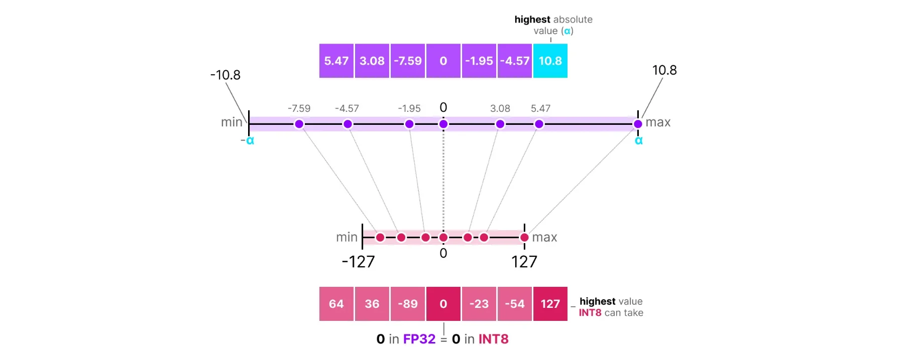 Source: https://newsletter.maartengrootendorst.com/p/a-visual-guide-to-quantization
scale = max(|W|) / (2^(b-1) - 1)
zero_point = 0  (fixed)
W_quantized = round(W / scale)
W_dequantized = W_quantized × scale
Where W is the original weight and b is the number of bits. For 8-bit symmetric quantization, we map values to the range [-127, 127]. Since the zero point is fixed at 0, the quantization range is always centered around zero. The problem is if weights are not centered around zero, we waste bit range.
Asymmetric Quantization handles this by calculating the zero point based on actual data:
 Source: https://newsletter.maartengrootendorst.com/p/a-visual-guide-to-quantization
scale = (max(W) - min(W)) / (2^b - 1)
zero_point = round(-min(W) / scale)
W_quantized = round(W / scale) + zero_point
W_dequantized = (W_quantized - zero_point) × scale
Here the zero point shifts based on where the weights actually lie. This uses the full bit range regardless of where the weights are centered. For example, if all weights are positive, asymmetric quantization will shift the zero point to use the full [0, 255] range for 8-bit, while symmetric would waste half the range.
The problem with baseline methods: They treat all weights equally. But in neural networks, some weights matter much more than others. Quantizing important weights poorly can hurt model quality significantly. This is why we need smarter approaches.
AWQ (Activation-aware Weight Quantization)
AWQ was introduced by MIT and NVIDIA researchers in 2023. The key insight: not all weights contribute equally to the output. Some weights are multiplied by large activation values, so errors in these weights get amplified. AWQ protects these "salient" weights.
How It Works
For a weight W and activation X, the output is Y = W × X. If X is large, any error in W gets magnified. The figure below illustrates this:
 Source:
 The figure shows the evolution from basic quantization to AWQ:
- Round-to-nearest (RTN) quantization gives poor perplexity (43.2)
- Keeping just 1% of salient weights in FP16 based on activation distribution improves perplexity to 13.0, but mixed-precision breaks hardware efficiency
- AWQ's solution: scale weights before quantization based on average activation magnitude, controlled by α. This achieves the same 13.0 perplexity while keeping all weights in the same low-bit format
The second column of the activation matrix X has high magnitudes (shown in red). The corresponding column in the weight matrix is "salient" since errors here hurt more. Instead of keeping these weights in FP16, AWQ scales them up before quantization to reduce relative error.
Finding Salient Weights
AWQ identifies important weights by looking at activation magnitudes. In a linear layer with weight matrix W of shape (out_features, in_features), each column corresponds to an input channel. AWQ computes the average absolute activation for each input channel across a calibration dataset:
s_x = mean(|X|, dim=0) # shape: (in_features,)
Channels with high s_x values are important since errors in their corresponding weights have a bigger impact on the output.
Per-Channel Scaling
Instead of keeping some weights in higher precision (which complicates hardware), AWQ uses per-channel scaling: scale up important weights before quantization, then scale down activations to compensate:
Q(W × s) × (X / s) ≈ W × X
Where Q() is the quantization function, s is a per-channel scaling factor, and W × s scales each column of W by the corresponding element of s.
Scaling up important weights reduces their relative quantization error. If a weight is 0.001 and we scale it to 0.1 before quantization, the quantization step size becomes relatively smaller compared to the weight value.
The Role of Alpha (α)
AWQ introduces a hyperparameter α that controls how much activation magnitude influences the scaling factor:
s = s_x^α
At different alpha values:
- α = 0: No scaling. AWQ becomes equivalent to standard quantization.
- α = 1: Scaling factor equals activation magnitude. Maximum protection for salient weights, but might over-scale some channels.
- 0 < α < 1: A balance. In practice, AWQ searches for the optimal α (typically around 0.5) that minimizes quantization error.
The Optimization Problem
AWQ searches for the optimal scaling factor s that minimizes output error:
L(s) = ||Q(W × diag(s)) × (diag(s)^(-1) × X) - W × X||²
Where:
W × diag(s): Scale each column of W by the corresponding element of sQ(...): Quantize the scaled weightsdiag(s)^(-1) × X: Scale down activations to compensateW × X: The original output we want to match
In practice, AWQ parameterizes s using alpha and performs a grid search:
s* = argmin_α ||Q(W × diag(s_x^α)) × (diag(s_x^(-α)) × X) - W × X||²
This search happens layer by layer during calibration.
The Full AWQ Process
- Calibration: Run a small dataset (128-512 samples) through the model and collect activation statistics
s_xfor each layer - Search: For each layer, find optimal α that minimizes
L(s) - Scale: Multiply weights by
s = s_x^α - Quantize: Apply asymmetric group-wise quantization to scaled weights
- Store: Save quantized weights along with scaling factors
During inference, activations are divided by s before matrix multiplication with quantized weights.
GPTQ (General Post-Training Quantization)
GPTQ was introduced in 2022 by researchers from IST Austria and ETH Zurich. It builds on the Optimal Brain Quantization (OBQ) framework but makes it practical for large models. The core idea differs from AWQ: GPTQ quantizes weights one at a time and adjusts remaining weights to compensate for the error introduced. It uses second-order information (the Hessian matrix) to determine which weights are most sensitive.
How It Works
For a layer with weights W and input X, we want the output to stay the same after quantization. The challenge: when we quantize a weight, we introduce error. GPTQ's insight is that we can adjust the remaining unquantized weights to compensate. To do this effectively, we need to understand how each weight affects the output, which is where the Hessian comes in.
Why Second-Order Information?
First-order information (gradients) tells us how much the loss changes if we adjust a weight slightly. But in quantization, we're not training. We're forced to change weights to discrete values and need to know how to adjust other weights to compensate.
Second-order information (Hessian) tells us how weights interact with each other. If we change weight i, what's the optimal change for weight j? This captures the relationship between different weights, which is exactly what we need for error compensation.
Consider a simple example with two weights w₁ and w₂. If we quantize w₁ and introduce error δ₁, first-order information doesn't tell us how to compensate using w₂. But the Hessian captures the relationship between w₁ and w₂, letting us compute exactly how much to adjust w₂ based on the error in w₁.
GPTQ assumes the loss function is approximately quadratic around the current weights. At a trained model, we're near a minimum, so the gradient is approximately zero and the loss change is dominated by the quadratic term involving the Hessian. This is why the Hessian matters: it captures how the loss curves around our current point and tells us how to minimize the cost of quantization.
The Hessian Matrix
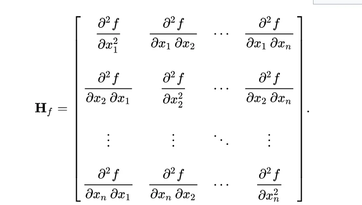 Source: https://en.wikipedia.org/wiki/Hessian_matrix
For a layer with squared error loss, the Hessian is H = 2 × X × X^T, where X is the input activation matrix collected during calibration. The Hessian has shape (in_features, in_features).
What does H represent?
- Diagonal elements H[i][i]: How sensitive the output is to weight column i. Large value means the column is important.
- Off-diagonal elements H[i][j]: How weight columns i and j interact. Non-zero value means changing one affects the optimal value of the other.
Second-order methods are more expensive (quadratic space and time complexity). For a layer with 4096 input features, the Hessian is a 4096×4096 matrix (67 million elements). GPTQ uses Cholesky decomposition and lazy batching to make this practical. Despite the cost, the quality improvement is worth it since quantization is a one-time process.
Group-wise Quantization
GPTQ uses group-wise quantization instead of pure row-wise. This divides each row into groups of g consecutive weights (typically g=128) and computes separate scale/zero-point for each group.
Why group-wise? Within a row, weights can have varying distributions. A row might have small values at the beginning and large values at the end. A single row-wise scale would be dominated by large values, causing poor precision for small values. Group-wise quantization adapts to local weight distributions at the cost of more storage for scales and zero-points.
Column-wise Weight Quantization
After computing the quantization grid (scale and zero-point) row by row, GPTQ quantizes the actual weights column by column. This is the core of GPTQ's algorithm.
Why column by column?
- When we quantize weight at column i, we introduce error
- We compensate by adjusting weights in columns i+1, i+2, ... (columns we haven't quantized yet)
- We can't adjust columns 0, 1, ..., i-1 because they're already quantized
Important distinction:
- Quantization grid (scale, zero-point): Calculated row by row (or group by group)
- Actual weight quantization: Done column by column with error compensation
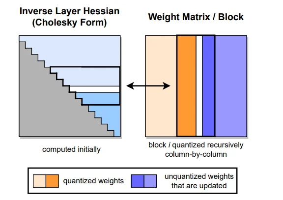 Source:
 The figure shows GPTQ's column-by-column quantization with Hessian-based error compensation. Left: The inverse Hessian in Cholesky form (lower triangular), computed once at the start. Right: The weight matrix being quantized block by block. Orange columns are already quantized. Blue columns are unquantized weights that get updated to compensate for quantization errors. The block structure enables lazy batching: local updates within a block, global updates to future blocks.
Error Calculation and Weight Updates
When we quantize a weight at column q, the quantization error δ_q is the difference between the original and quantized value. The increase in squared error is proportional to δ_q² × H[q][q]. If H[q][q] is large, even a small quantization error causes big output error.
After quantizing weight at column q, we reduce total error by adjusting remaining unquantized weights. The optimal adjustment for weight at column i (where i > q) is:
w_i = w_i - (δ_q / H[q][q]) × H[q][i]
Where δ_q is the quantization error, H[q][q] is the diagonal Hessian element (sensitivity), and H[q][i] is the off-diagonal element (interaction strength). This formula comes directly from the Hessian and is the mathematically optimal way to compensate for quantization error.
Lazy Batching
The basic algorithm quantizes one column at a time, which is slow due to memory operations. GPTQ introduces lazy batching:
- Quantize a batch of B columns (typically B=128)
- Accumulate all update terms
- Apply all updates at once
This reduces memory operations by a factor of B and improves GPU utilization.
GPTQ distinguishes between local updates (within a batch, applied immediately) and global updates (across batches, applied at batch boundaries). For numerical stability, GPTQ uses Cholesky decomposition (H = L × L^T) instead of directly computing the Hessian inverse.
The Complete GPTQ Process
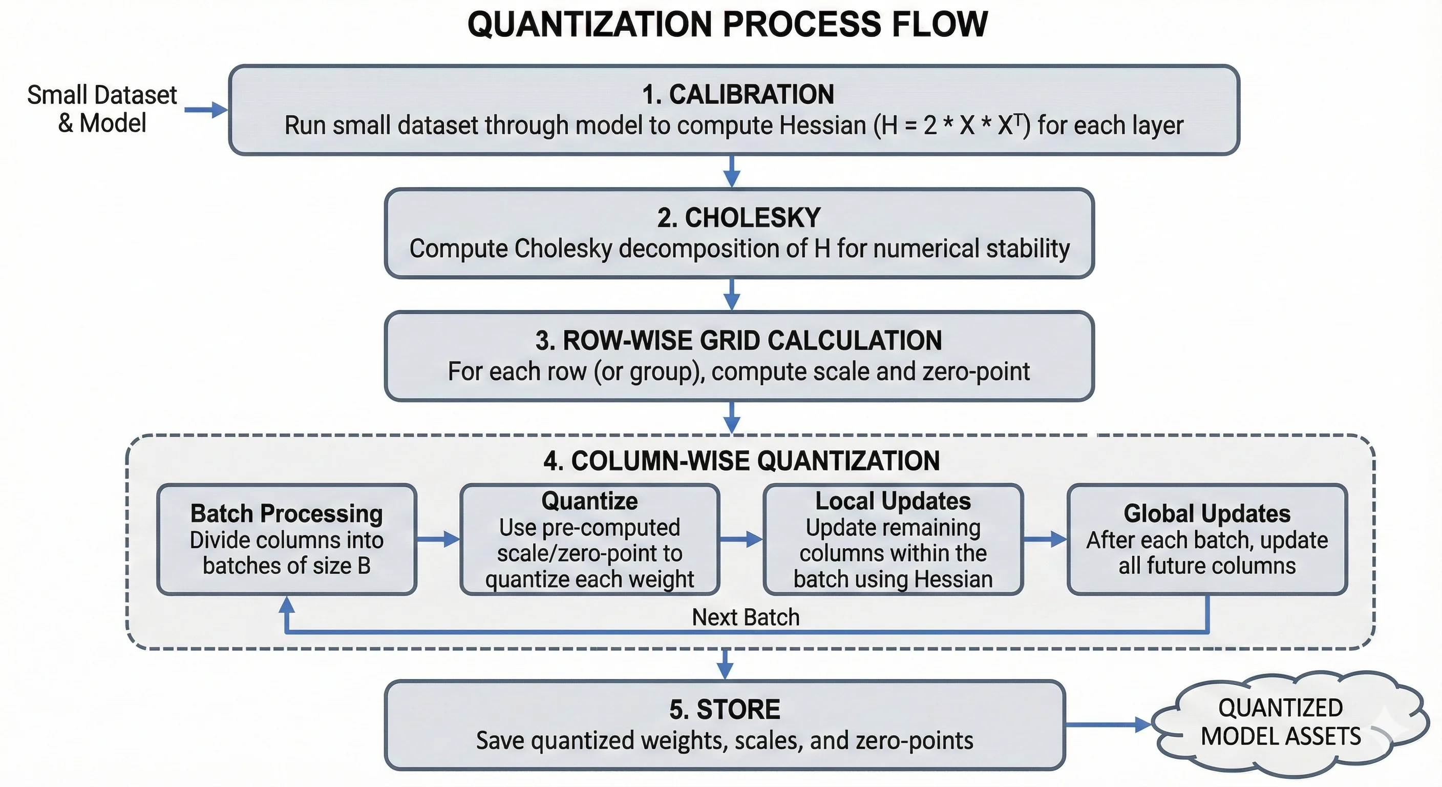 Source: Generated by Nano Banana Pro
- Calibration: Run a small dataset (128-1024 samples) through the model to compute the Hessian for each layer
- Cholesky: Compute Cholesky decomposition of H for numerical stability
- Row-wise grid calculation: For each row (or group), compute scale and zero-point
- Column-wise quantization: Process columns left to right in batches:
- Quantize using pre-computed scale/zero-point
- Apply local updates within the batch
- Apply global updates to future columns after each batch
- Store: Save quantized weights, scales, and zero-points
Quantization Type: Asymmetric, group-wise (group size typically 128), supports 4-bit and 8-bit.
Marlin
Marlin is not a quantization algorithm. It's a highly optimized CUDA kernel for running already-quantized models (GPTQ/AWQ) faster. Developed by IST Austria (the same group behind GPTQ), Marlin runs matrix multiplication on NVIDIA GPUs with close to ideal memory bandwidth utilization.
In our benchmarks, we tested Marlin with both GPTQ and AWQ quantized models:
- Marlin-GPTQ: Used
Qwen/Qwen2.5-32B-Instruct-GPTQ-Int4- achieved 712 tok/s compared to GPTQ's 276 tok/s, a 2.6x speedup - Marlin-AWQ: Used
Qwen/Qwen2.5-32B-Instruct-AWQ- achieved 741 tok/s compared to AWQ's 68 tok/s, a 10.9x speedup
The only difference was the kernel used for inference. The quantized weights remained the same, demonstrating how much kernels matter for performance.
Why Is Marlin So Fast?
To understand Marlin's speed, we need to understand GPU memory hierarchy and why standard GPTQ inference is slow.
Modern GPUs like H200 have a hierarchical memory system. From slowest to fastest:
- DRAM/HBM: 141 GB capacity, ~4.8 TB/s bandwidth. Main memory with high capacity but relatively slow access.
- L2 Cache: 50 MB on H200, shared across all SMs. ~12 TB/s bandwidth.
- L1 Cache / Shared Memory (SMEM): 256 KB per SM, private to each SM. ~19 TB/s bandwidth.
- Registers (RF): 256 KB per SM, fastest access with direct connection to compute units.
- Tensor Core Units (TCUs): Where actual computation happens.
The key insight: moving data between these levels is expensive. The goal is to maximize cache hits and minimize cache misses.
The Problem with Standard GPTQ Inference
Standard GPTQ inference loads quantized weights from HBM, dequantizes them to FP16, performs matrix multiplication, and repeats. The problem is a memory bandwidth bottleneck: compute units wait for data from HBM.
Issues with the standard approach:
- Poor data reuse: Weights are loaded, used once, then discarded
- Cache misses: Data access patterns don't align with cache structure
- Synchronous execution: Compute units wait while data is being fetched
- Inefficient dequantization: Dequantize happens in the critical path
How Marlin Solves This
1. Asynchronous Copy (Async-Copy)
Traditional GPU memory operations are synchronous, meaning compute units wait while data loads. Async-copy allows memory operations to happen in parallel with computation.
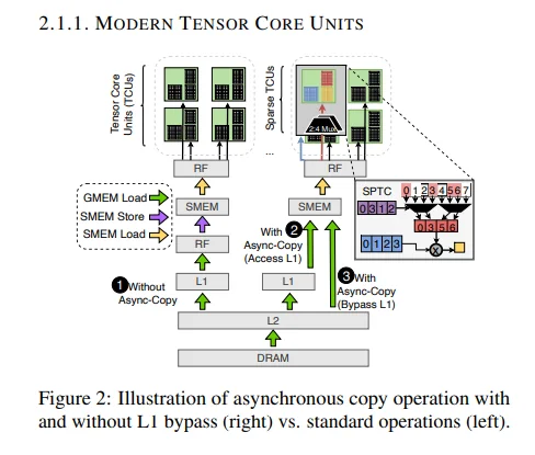 Source:
 The figure shows three approaches:
-
Without Async-Copy: Data flows synchronously from DRAM through L2 and L1 to shared memory, then to registers and tensor cores. Each step waits for the previous one, causing L1 cache pollution and idle tensor cores during loads.
-
With Async-Copy (Access L1): Loads happen asynchronously while tensor cores work on previous data. However, data still goes through L1, causing some cache pollution.
-
With Async-Copy (Bypass L1): What Marlin uses. Data flows from DRAM through L2 directly to shared memory, bypassing L1. This keeps L1 free for activations, provides lower latency, and ensures full overlap of memory operations with compute.
2. Optimized L2 Cache Utilization
Marlin organizes data access patterns to maximize L2 cache hits. Standard GPTQ has random access patterns achieving 30-50% cache hit rates. Marlin uses streaming access patterns that keep weights in L2 for multiple uses, achieving 80-95% hit rates.
Marlin processes weights in a specific order ensuring that when a weight is loaded into L2, it's used multiple times before eviction. Adjacent weights are accessed together (spatial locality), and the same weights are accessed again soon (temporal locality).
3. Shared Memory (SMEM) Optimization
Marlin uses shared memory as a software-managed cache with double buffering. While one tile of weights is being used for computation, the next tile loads asynchronously. This creates a pipeline where compute never stalls waiting for data.
Key techniques:
- Double buffering: Load tile B while computing on tile A
- Coalesced access: All threads in a warp access consecutive memory addresses
- Bank conflict avoidance: Data layout prevents shared memory bank conflicts
4. Efficient Dequantization
Standard GPTQ dequantizes weights in separate steps: load 4-bit weight, dequantize to FP16 in a separate kernel, store FP16 weight, load it again for matrix multiplication, then compute.
Marlin fuses dequantization with computation: load 4-bit weight asynchronously while bypassing L1, then dequantize and compute in the same fused kernel. This eliminates extra memory round-trips, kernel launch overhead, and intermediate storage.
5. Warp-Level Parallelism
Marlin efficiently distributes work across GPU threads. A streaming multiprocessor contains multiple warps (32 threads each) that feed into tensor cores. Marlin ensures all threads in a warp access memory together (coalesced access), work is evenly distributed across warps, and there's no warp divergence.
6. Sparse Tensor Core Utilization
Modern GPUs have Sparse Tensor Core Units for accelerating sparse matrix operations. While standard Marlin focuses on dense operations, the architecture is designed to potentially leverage sparsity in future versions.
BitBLAS
BitBLAS is developed by Microsoft as part of their TileLang project. Like Marlin, BitBLAS is not a quantization algorithm. It's a kernel generation library that creates highly optimized CUDA kernels for low-bit matrix operations. Think of it as a compiler that takes your quantization configuration and generates custom GPU code for your specific hardware and matrix sizes.
The key insight: generic CUDA kernels can't be optimal for all situations. Different GPUs, matrix sizes, and quantization formats need different optimization strategies. BitBLAS solves this by generating specialized kernels on-the-fly.
Kernel Builder Architecture
BitBLAS uses a multi-stage process to generate optimized kernels:
- DSL Definition: Define your matrix operation using TensorIR (a domain-specific language) that describes what computation you want, not how to do it.
- Tiling Strategy: Divide matrices into small blocks (tiles) sized based on your GPU's resources.
- Optimization Search: Search through different optimization strategies (Ladder Optimization) to find the fastest configuration.
- Code Generation: Compile the optimized schedule into CUDA code.
- Caching: Cache generated kernels so the search only happens once per configuration.
TensorIR: Domain-Specific Language
BitBLAS uses TensorIR (part of Apache TVM) to define computations. TensorIR separates "what to compute" from "how to compute it."
When you write matrix multiplication in Python or C++, you specify both computation and loop structure, making optimization difficult. TensorIR separates these concerns:
- Computation definition: What values to compute (element-wise formulas)
- Schedule: How to organize the computation (loop order, parallelization, memory placement)
For quantized matmul, BitBLAS defines these computation stages:
- Load: Read quantized weights, scales, zero-points from global memory
- Unpack: Extract 4-bit values from packed 8-bit storage
- Dequantize: Convert to FP16 using scale and zero-point
- Compute: Perform matrix multiplication
- Store: Write results back to global memory
TensorIR lets BitBLAS express this computation once, then search for the best schedule for your hardware.
Tiles: The Building Blocks
Tiles are small blocks of input matrices that fit into fast GPU memory. Instead of processing entire matrices at once, BitBLAS processes tile by tile. For C = A × B:
- Matrix A is divided into tiles of size (tile_M, tile_K)
- Matrix B is divided into tiles of size (tile_K, tile_N)
- Output C is computed in tiles of size (tile_M, tile_N)
Tiling allows data reuse in fast memory. Without tiling, each element would be loaded from slow global memory multiple times. With tiling, we load once into shared memory and reuse many times.
BitBLAS automatically selects tile sizes based on:
- Shared memory capacity: Tiles must fit (e.g., 256KB per SM on H100)
- Register pressure: Partial results must not exceed register file size
- Tensor core alignment: Dimensions must align with tensor core requirements (typically multiples of 16)
- Occupancy: Smaller tiles allow more thread blocks to run concurrently
Typical tile sizes for 4-bit quantized matmul: tile_M/N of 128 or 256, tile_K of 32 or 64.
Hardware Awareness
BitBLAS queries your GPU's specifications and adjusts accordingly. Properties it considers:
- Compute capability (available instructions, tensor cores)
- Shared memory and register file size
- Warp size (32 on NVIDIA) and SM count
- Memory bandwidth and tensor core type
Ladder Optimization
Ladder Optimization is BitBLAS's auto-tuning strategy. For a quantized matmul kernel, there are many choices: tile sizes, thread block configuration, shared memory layout, pipeline depth, loop unrolling. The total combinations can be in the millions.
Instead of exhaustive search, Ladder Optimization uses a hierarchical approach:
- Coarse search: Try a small set of tile sizes, pick top performers
- Thread block tuning: For each good tile size, search thread configurations
- Memory optimization: Tune shared memory layout and bank conflict avoidance
- Instruction scheduling: Optimize instruction order for latency hiding
- Fine tuning: Adjust pipeline depth, unrolling, etc.
Each level refines choices from the previous level, dramatically reducing the search space. BitBLAS also uses a cost model (estimating memory bandwidth, compute utilization, cache hit rates) to guide the search without actually running every configuration.
Caching and Reuse
Once BitBLAS finds an optimized kernel for a configuration, it caches the result. Future calls reuse the cached kernel instantly. The cache key includes matrix dimensions, quantization format, data types, and GPU architecture.
BitsandBytes
BitsandBytes was created by Tim Dettmers, initially for 8-bit optimizers and later expanded to inference quantization. Unlike AWQ and GPTQ which require pre-quantized model files, BitsandBytes quantizes on-the-fly during model loading. You can take any model and load it in 4-bit or 8-bit without any preparation.
BitsandBytes supports two 4-bit data types: NF4 (NormalFloat4) and FP4 (FloatingPoint4).
NF4 vs FP4
FP4 (FloatingPoint4) is a standard 4-bit floating point format using 1 sign bit, 2 exponent bits, and 1 mantissa bit. Quantization levels are uniformly spaced in log scale, making it suitable for data with any distribution.
NF4 (NormalFloat4) is designed specifically for neural network weights. It assumes weights follow a normal (Gaussian) distribution and places quantization levels where most weights are concentrated (near zero). Neural network weights cluster around zero in a bell curve, so NF4 puts more quantization levels there, resulting in less error. FP4 wastes levels in the tails where few weights exist.
How It Works
BitsandBytes quantization involves four steps:
Step 1: Block Splitting - Weights are split into small blocks (typically size 64), each processed independently. Different parts of the weight matrix can have different scales, so block-wise processing allows local adaptation at the cost of more storage for absmax values.
Step 2: Absmax Extraction - For each block, find the maximum absolute value (absmax). This normalizes the block to the range [-1, 1] by dividing each value by absmax.
Step 3: Quantization Using Lookup Tables - Each normalized weight is mapped to the nearest value in a predefined lookup table.
NF4 Lookup Table (16 values, computed from quantiles of standard normal distribution):
| 4-bit Index | NF4 Value |
|---|---|
| 0 | -1.0 |
| 1 | -0.6961928009 |
| 2 | -0.5250730514 |
| 3 | -0.3949584961 |
| 4 | -0.2844238281 |
| 5 | -0.1848487854 |
| 6 | -0.0911179781 |
| 7 | 0.0 |
| 8 | 0.0796291083 |
| 9 | 0.1609346867 |
| 10 | 0.2461108565 |
| 11 | 0.3379120827 |
| 12 | 0.4407081604 |
| 13 | 0.5626170039 |
| 14 | 0.7229568362 |
| 15 | 1.0 |
Notice how levels are denser near zero and sparser at extremes.
FP4 Lookup Table (uniformly spaced in log scale, sign handled separately):
| 4-bit Index | FP4 Value |
|---|---|
| 0 | 0.0 |
| 1 | 0.0625 |
| 2 | 0.125 |
| 3 | 0.1875 |
| 4 | 0.25 |
| 5 | 0.3125 |
| 6 | 0.375 |
| 7 | 0.4375 |
| 8 | 0.5 |
| 9 | 0.625 |
| 10 | 0.75 |
| 11 | 0.875 |
| 12 | 1.0 |
| 13 | 1.25 |
| 14 | 1.5 |
| 15 | 2.0 |
For each normalized weight, find the nearest lookup table value and store its index. For example, if a normalized weight is 0.35, compare distances to nearby NF4 values: index 10 (0.2461) has distance 0.1039, index 11 (0.3379) has distance 0.0121, index 12 (0.4407) has distance 0.0907. The closest is index 11, so we store the 4-bit value 11.
Step 4: Dequantization - During inference, recover approximate FP16 values by looking up the index in the table and multiplying by the stored absmax. If we stored index 11 with absmax 0.67, we get 0.3379 × 0.67 = 0.2264 (original was ~0.2345).
Double Quantization
BitsandBytes supports double quantization, which quantizes the absmax values themselves. In standard quantization, absmax uses FP32 (32 bits) per block, adding 0.5 bits per weight overhead for block size 64. With double quantization, absmax is quantized to 8 bits, reducing overhead to 0.125 bits per weight with minimal quality impact.
NF4 vs FP4: When to Use Which?
| Aspect | NF4 | FP4 |
|---|---|---|
| Best for | Neural network weights | General data |
| Assumption | Weights are normally distributed | No assumption |
| Precision near zero | High (dense levels) | Medium (uniform) |
| Precision at extremes | Lower (sparse levels) | Medium (uniform) |
| Typical use | LLM inference | Mixed workloads |
Recommendation: Use NF4 for LLM inference. Most neural network weights follow a roughly normal distribution, so NF4's optimized quantization levels provide better precision.
Calibration: No calibration needed. Quantization happens at runtime during model loading.
Quantization Type: Symmetric, block-wise (default block size of 64).
Current vLLM Limitation: vLLM doesn't currently support 8-bit BitsandBytes. There's an open GitHub issue (#8799) tracking this.
GGUF (GPT-Generated Unified Format)
GGUF was created by the llama.cpp project, led by Georgi Gerganov. It's the successor to the older GGML format. Important clarification: GGUF is not a quantization algorithm. It's a file format (container) that stores quantized weights along with model metadata. The actual quantization uses standard techniques (scale and zero-point) but with a clever block and sub-block structure.
- AWQ, GPTQ: Quantization algorithms (how to quantize)
- GGUF: File format + standard quantization (how to store + basic quantization)
The GGUF File Format
GGUF is a binary file format designed to be:
- Self-contained: All model information in one file (weights, tokenizer, config)
- Portable: Works across different hardware and software
- Extensible: Easy to add new metadata fields
- Memory-mappable: Can load directly without parsing
GGUF File Structure:
The file starts with a magic number "GGUF" (4 bytes) followed by a version number (uint32), tensor count and metadata key-value count (both uint64).
The metadata section contains key-value pairs like general.architecture, general.name, llama.context_length, llama.embedding_length, llama.block_count, and tokenizer info.
After metadata, tensor info is stored for each tensor including name (e.g., "blk.0.attn_q.weight"), dimensions (e.g., [5120, 5120]), quantization type (e.g., Q4_K), and offset pointer to actual data. Finally, the tensor data section contains the quantized weights in binary format, aligned for efficient memory access.
GGUF Quantization Types
GGUF supports many quantization types differing in bits per weight, block structure, and quality:
| Type | Bits | Block Size | Description |
|---|---|---|---|
| Q4_0 | 4 | 32 | Basic 4-bit, no sub-blocks |
| Q4_1 | 4 | 32 | 4-bit with min value stored |
| Q5_0 | 5 | 32 | 5-bit quantization |
| Q5_1 | 5 | 32 | 5-bit with min value stored |
| Q8_0 | 8 | 32 | 8-bit quantization |
| Q4_K | 4 | 256 | K-quant 4-bit with sub-blocks |
| Q5_K | 5 | 256 | K-quant 5-bit with sub-blocks |
| Q6_K | 6 | 256 | K-quant 6-bit with sub-blocks |
| Q4_K_M | 4 | 256 | K-quant 4-bit, medium quality |
| Q5_K_M | 5 | 256 | K-quant 5-bit, medium quality |
| Q4_K_S | 4 | 256 | K-quant 4-bit, small (faster) |
| Q5_K_S | 5 | 256 | K-quant 5-bit, small (faster) |
The "K-quants" (Q4_K, Q5_K, etc.) are the most advanced, using a block + sub-block structure for better quality.
How GGUF Quantization Works
GGUF uses block-based quantization with a hierarchical structure. Basic types (Q4_0, Q8_0) use symmetric quantization, while K-quants (Q4_K, Q4_K_M) use asymmetric quantization, storing both scales and minimums at the block and sub-block levels.
Step 1: Block Creation - Weights are divided into blocks. For K-quants, the block size is typically 256 weights. Block 0 contains weights 0-255, Block 1 contains weights 256-511, and so on.
Step 2: Sub-block Creation (K-quants only) - Each block is further divided into sub-blocks for finer granularity. With block size 256 and sub-block size 32, each block contains 8 sub-blocks. Sub-blocks allow finer adaptation to local weight distributions with minimal overhead.
Step 3: Scale and Zero-Point Calculation - At the block level, the scale d is computed as max absolute value divided by half the quantization range (7.5 for 4-bit). For K-quants, each sub-block gets its own scale stored relative to the block scale to save space. Sub-block mins are also stored for asymmetric quantization.
Q4_K Block Structure:
For Q4_K, each block of 256 weights stores:
- Block scale (d): FP16, 2 bytes
- Block min (dmin): FP16, 2 bytes
- Sub-block scales: 8 values × 6-bit = 6 bytes
- Sub-block mins: 8 values × 6-bit = 6 bytes
- Quantized weights: 256 values × 4-bit = 128 bytes
Total per block: 2 + 2 + 6 + 6 + 128 = 144 bytes = 4.5 bits/weight effective
Step 4: Quantization Process - For each weight in a sub-block:
- Subtract the sub-block min
- Divide by (block_scale × sub_block_scale) to normalize
- Multiply by max integer value (15 for 4-bit)
- Round to nearest integer and clamp to [0, 15]
For example, weight 0.12 with block_scale=0.67, sub_block_scale=0.672, sub_block_min=-0.45:
- Subtract min: 0.12 - (-0.45) = 0.57
- Normalize: 0.57 / (0.67 × 0.672) = 1.267
- Scale to int: 1.267 × 15 = 19.0
- Clamp: min(max(19, 0), 15) = 15
Two 4-bit values are packed into each byte.
Step 5: Dequantization - During inference, reverse the process:
- Divide quantized int by max value (15 for 4-bit)
- Multiply by block_scale × sub_block_scale
- Add back sub_block_min
For dequantizing value 15: 15/15 = 1.0, then 1.0 × 0.67 × 0.672 = 0.45, plus min (-0.45) = 0.0. The original was 0.12, so there's some quantization error.
Quantization Types Explained
Q4_0 (Basic 4-bit): Block size 32 weights. Stores FP16 scale (2 bytes) + 32 weights at 4-bit (16 bytes) = 18 bytes = 4.5 bits/weight. Symmetric quantization with no zero-point. Dequantized weight = scale × (q - 8), where q is in [0,15] centered at 8.
Q4_1 (4-bit with min): Block size 32 weights. Stores FP16 scale (2 bytes) + FP16 min (2 bytes) + 32 weights (16 bytes) = 20 bytes = 5.0 bits/weight. Asymmetric quantization. Dequantized weight = scale × q + min.
Q4_K (K-quant 4-bit): Block size 256 with 8 sub-blocks of 32 each. Stores block scale/min, sub-block scales/mins (6-bit each), and weights = 144 bytes = 4.5 bits/weight. The hierarchical structure provides better precision than flat Q4_0 because each sub-block adapts to local weight distributions.
Q5_K_M (K-quant 5-bit medium): Block size 256 with 8 sub-blocks, 5 bits per weight. The 5th bit is stored separately for efficient packing = 176 bytes = 5.5 bits/weight. The "_M" suffix indicates medium quality; "_S" variants are smaller/faster but lower quality.
TorchAO (Torch Architecture Optimization)
TorchAO is PyTorch's native quantization toolkit developed by the PyTorch team at Meta. It provides various quantization schemes including int4 weight-only quantization and integrates directly with PyTorch's compilation stack (torch.compile). The goal is to make quantization a first-class citizen in PyTorch without requiring external libraries.
Unlike AWQ and GPTQ which use sophisticated algorithms, TorchAO uses straightforward asymmetric quantization but leverages PyTorch's native operations and compiler optimizations for speed.
Weight-Only Quantization
TorchAO implements int4 weight-only quantization: weights are quantized to 4-bit integers while activations remain in FP16 or BF16.
Why weight-only for LLMs?
- LLM inference is memory-bound, not compute-bound
- Reducing weight size from 16-bit to 4-bit cuts memory bandwidth by 4x
- Activations are dynamic and harder to quantize accurately
- Weight-only avoids the quality loss from activation quantization
Quantization Process
Step 1: Group Creation - TorchAO divides weights into groups along the input channel dimension. Default group size is 128. For a weight matrix of shape (4096, 4096) with group_size=128: 32 groups per row × 4096 rows = 131,072 groups, each with 128 weights sharing one scale and zero-point.
Step 2: Finding Min and Max - For each group, find group_min and group_max to define the range mapped to 4-bit integers.
Step 3: Scale and Zero-Point Calculation - TorchAO uses asymmetric quantization. For 4-bit, the integer range is [0, 15]:
scale = (group_max - group_min) / 15
zero_point = clamp(round(-group_min / scale), 0, 15)
Example: Group with weights ranging from -0.8 to 0.4:
- scale = (0.4 - (-0.8)) / 15 = 0.08
- zero_point = round(0.8 / 0.08) = 10
- Integer 0 → -0.8, Integer 10 → 0.0, Integer 15 → 0.4
Step 4: Quantization - Each weight is quantized:
quantized_weight = clamp(round(weight / scale) + zero_point, 0, 15)
Examples with scale=0.08, zero_point=10:
- Weight -0.8 → round(-10) + 10 = 0
- Weight 0.0 → 0 + 10 = 10
- Weight 0.4 → 5 + 10 = 15
- Weight -0.24 → -3 + 10 = 7
Step 5: Packing - Two 4-bit integers pack into one byte. Even indices go into lower 4 bits, odd indices into upper 4 bits. For weights [7, 12, 3, 15]: Byte 0 = (12 << 4) | 7 = 0xC7, Byte 1 = (15 << 4) | 3 = 0xF3.
Step 6: Dequantization - During inference, weights are dequantized on-the-fly:
dequantized_weight = (quantized_weight - zero_point) × scale
Example: Quantized=7, zero_point=10, scale=0.08 → (7-10) × 0.08 = -0.24 ✓
Memory Layout
For weight matrix (out_features, in_features) with group_size=128:
- Quantized weights: (out_features, in_features/2) in uint8 (each byte holds two 4-bit weights)
- Scales: (out_features, in_features/128) in FP16 (one per group)
- Zero-points: (out_features, in_features/128) in int4 or int8 (one per group)
TorchAO Quantization Types
| Type | Bits | Group Size | Description |
|---|---|---|---|
| int4_weight_only | 4 | 128 | Default int4, good balance |
| int4_weight_only (group=32) | 4 | 32 | Smaller groups, higher quality |
| int4_weight_only (group=256) | 4 | 256 | Larger groups, more compression |
| int8_weight_only | 8 | Per-channel | 8-bit quantization |
| int8_dynamic | 8 | Dynamic | Weight + activation quantization |
For LLM inference, int4_weight_only with group_size=128 is most common.
Integration with PyTorch Compiler
TorchAO works seamlessly with torch.compile. When you quantize and compile:
- Fusion: Dequantization is fused with matrix multiplication
- Kernel optimization: PyTorch generates optimized CUDA kernels
- Memory planning: Efficient memory allocation for quantized tensors
This compiler integration differentiates TorchAO from standalone quantization libraries.
Current vLLM Status
During our experiments, we encountered issues getting TorchAO to work with vLLM. The engine didn't recognize the torchao_config parameter. This appears to be a bug in the vLLM project.
LLM Benchmark Setup: Experiments & Configuration
In this section, we'll cover what model we used, what hardware we ran on, and how we measured performance. All our experiments focus on 4-bit quantization.
Model and Hardware
Model: Qwen2.5-32B-Instruct
Hardware: NVIDIA H200 GPU
We ran all experiments on H200 with 140GB memory. This is important to note because some quantization techniques are hardware-dependent. For example, BitBLAS doesn't work on H200 (it's optimized for A100).
Getting the Hardware
To run these experiments, we used JarvisLabs. Here's how to set up your own instance:
- Log in to JarvisLabs and navigate to the dashboard.
- Create an Instance: Click Create and select your desired GPU configuration.
- Select Your GPU:
- Choose H200 for higher performance.
- Choose the Framework: Select PyTorch from the available frameworks.
- Launch: Click Launch. Your instance will be ready in a few minutes.
Pre-quantized Models We Used
For 4-bit quantization, we used these checkpoints:
| Technique | HuggingFace Model ID | Notes |
|---|---|---|
| Baseline (FP16) | Qwen/Qwen2.5-32B-Instruct | No quantization |
| AWQ | Qwen/Qwen2.5-32B-Instruct-AWQ | Official AWQ checkpoint |
| GPTQ | Qwen/Qwen2.5-32B-Instruct-GPTQ-Int4 | Official GPTQ checkpoint |
| Marlin-GPTQ | Qwen/Qwen2.5-32B-Instruct-GPTQ-Int4 | Uses GPTQ checkpoint with Marlin kernel |
| Marlin-AWQ | Qwen/Qwen2.5-32B-Instruct-AWQ | Uses AWQ checkpoint with Marlin kernel |
| GGUF | Qwen/Qwen2.5-32B-Instruct-GGUF | Q4_K_M variant |
| BitsandBytes | Qwen/Qwen2.5-32B-Instruct | Quantizes on-the-fly |
Note: BitBLAS and TorchAO were excluded. BitBLAS doesn't support H200, and TorchAO had config issues with vLLM.
Evaluation Framework: lm-evaluation-harness
For running perplexity and HumanEval benchmarks, we used lm-evaluation-harness (also known as lm_eval). It's an open-source framework developed by EleutherAI for evaluating language models.
Why we chose it:
- Supports 200+ benchmarks out of the box (Wikitext, HumanEval, MMLU, etc.)
- Works directly with vLLM as a backend
- Handles all the data loading, prompting, and metric calculation
- Widely used in the community, so results are comparable
Installation is simple:
pip install lm_eval
The framework lets us specify vLLM as the model backend using --model vllm, and we can pass vLLM-specific arguments like quantization method and GPU memory utilization through --model_args.
Datasets and Metrics
We measured three things: model quality (perplexity), code generation ability, and inference speed.
1. Perplexity - Wikitext-2
What it measures: How well the model predicts text. Lower is better.
Dataset: Wikitext-2 is a collection of Wikipedia articles. The model tries to predict the next word, and we measure how surprised it is by the actual answer.
Why it matters: Perplexity tells us if quantization hurt the model's language understanding. A big jump in perplexity means the model got dumber.
2. Code Generation - HumanEval
What it measures: Can the model write working code?
Dataset: HumanEval was created by OpenAI to evaluate code generation capabilities. It contains 164 hand-written Python programming problems. Each problem has:
- A function signature and docstring describing the task
- A canonical solution (hidden during evaluation)
- Unit tests to check if the code works
Here's an example problem from HumanEval:
{
  "task_id": "HumanEval/0",
  "prompt": "from typing import List\n\ndef has_close_elements(numbers: List[float], threshold: float) -> bool:\n    \"\"\" Check if in given list of numbers, are any two numbers closer to each other than given threshold.\n    >>> has_close_elements([1.0, 2.0, 3.0], 0.5)\n    False\n    >>> has_close_elements([1.0, 2.8, 3.0, 4.0, 5.0, 2.0], 0.3)\n    True\n    \"\"\"\n",
  "entry_point": "has_close_elements",
  "test": "def check(candidate):\n    assert candidate([1.0, 2.0, 3.9, 4.0, 5.0, 2.2], 0.3) == True\n    ..."
}
Metric: Pass@1 - the percentage of problems the model solves correctly on the first try.
Pass@1 = Number of problems solved correctly / Total problems (164)
Why it matters: Code generation is a demanding task. If quantization breaks something subtle in the model's reasoning, it will show up here.
3. Inference Speed - ShareGPT
What it measures: How fast can the model generate responses?
Dataset: ShareGPT contains real conversations between users and ChatGPT. We use 200 prompts from this dataset.
Metrics:
- Throughput (tok/s): Total tokens generated per second
- TTFT (ms): Time to First Token - how long until the first token appears
- ITL (ms): Inter-Token Latency - time between consecutive tokens
Why it matters: In production, speed matters. We want to know if quantization actually makes things faster.
Commands We Used
Here are the commands for running benchmarks:
1. lm_eval
This tool puts our model through a series of tests.
-
--model vllm: Tells the tool to use the vLLM engine to run the model. -
--model_args: This is a list of specific details for the model. -
pretrained=: The name or local folder path of our model (e.g.,Qwen/Qwen2.5-32B).
-
quantization=: Tells vLLM how the model was compressed (e.g.,awq,gptq, ormarlin).
-
gpu_memory_utilization=: A number between0.0and1.0. For example,0.8means "use 80% of my VRAM."
-
--tasks: The name of the test we want to run (e.g.,wikitextfor reading orhumanevalfor coding). -
--batch_size auto: This tells the tool to automatically figure out how many questions it can ask the model at once without crashing your GPU.
2. vllm serve
Before we can test speed, we need to deploy our model. vllm serve command by default deploys our model on localhost address having host 127.0.0.1 and port 8000.
[model name]: Usually the first thing afterserve, it's the folder or Hugging Face ID of the model.--quantization: Just like inlm_eval, this tells the server which compression "language" the model is using so it knows how to read it.--gpu-memory-utilization: Very important! If you are running multiple things on one GPU, set this lower (like0.5). If it’s the only thing running,0.8or0.9is usually safe.
3. vllm bench serve
This command sends a "flood" of fake users to your server to see when it starts to slow down.
--model: The name you want to give this model in the final report.--dataset-name sharegpt: Tells the tool to use a specific set of real-world user prompts.--dataset-path: The exact location of the.jsonfile containing those prompts.--max-concurrency 10: This simulates 10 people asking questions at the exact same time.--num-prompts 200: The total number of questions to send. Once 200 are finished, the test stops and gives you the results.
These are the actual commands I used for benchmarking all the techniques.
Perplexity (Wikitext-2)
# Baseline
lm_eval --model vllm \
  --model_args pretrained=Qwen/Qwen2.5-32B-Instruct,gpu_memory_utilization=0.8 \
  --tasks wikitext \
  --batch_size auto

# AWQ
lm_eval --model vllm \
  --model_args pretrained=Qwen/Qwen2.5-32B-Instruct-AWQ,gpu_memory_utilization=0.8,quantization=awq \
  --tasks wikitext \
  --batch_size auto

# GPTQ
lm_eval --model vllm \
  --model_args pretrained=Qwen/Qwen2.5-32B-Instruct-GPTQ-Int4,gpu_memory_utilization=0.8,quantization=gptq \
  --tasks wikitext \
  --batch_size auto

# Marlin-GPTQ
lm_eval --model vllm \
  --model_args pretrained=Qwen/Qwen2.5-32B-Instruct-GPTQ-Int4,gpu_memory_utilization=0.8,quantization=marlin \
  --tasks wikitext \
  --batch_size auto

# Marlin-AWQ
lm_eval --model vllm \
  --model_args pretrained=Qwen/Qwen2.5-32B-Instruct-AWQ,gpu_memory_utilization=0.8,quantization=marlin \
  --tasks wikitext \
  --batch_size auto

# GGUF
lm_eval --model vllm \
  --model_args pretrained=Qwen/Qwen2.5-32B-Instruct,model=qwen2.5-32b-instruct-q4_k_m.gguf,tokenizer=Qwen/Qwen2.5-32B-Instruct,quantization=gguf,gpu_memory_utilization=0.8 \
  --tasks wikitext \
  --batch_size auto

# BitsandBytes
lm_eval --model vllm \
  --model_args pretrained=Qwen/Qwen2.5-32B-Instruct,gpu_memory_utilization=0.8,quantization=bitsandbytes,load_format=bitsandbytes \
  --tasks wikitext \
  --batch_size auto
HumanEval
# Baseline
lm_eval --model vllm \
  --model_args pretrained=Qwen/Qwen2.5-32B-Instruct,gpu_memory_utilization=0.8 \
  --tasks humaneval \
  --confirm_run_unsafe_code \
  --batch_size auto

# AWQ
lm_eval --model vllm \
  --model_args pretrained=Qwen/Qwen2.5-32B-Instruct-AWQ,quantization=awq,gpu_memory_utilization=0.8 \
  --tasks humaneval \
  --confirm_run_unsafe_code \
  --batch_size auto

# GPTQ
lm_eval --model vllm \
  --model_args pretrained=Qwen/Qwen2.5-32B-Instruct-GPTQ-Int4,quantization=gptq,gpu_memory_utilization=0.8 \
  --tasks humaneval \
  --confirm_run_unsafe_code \
  --batch_size auto

# Marlin-GPTQ
lm_eval --model vllm \
  --model_args pretrained=Qwen/Qwen2.5-32B-Instruct-GPTQ-Int4,quantization=marlin,gpu_memory_utilization=0.8 \
  --tasks humaneval \
  --confirm_run_unsafe_code \
  --batch_size auto

# Marlin-AWQ
lm_eval --model vllm \
  --model_args pretrained=Qwen/Qwen2.5-32B-Instruct-AWQ,quantization=marlin,gpu_memory_utilization=0.8 \
  --tasks humaneval \
  --confirm_run_unsafe_code \
  --batch_size auto

# GGUF
lm_eval --model vllm \
  --model_args pretrained=Qwen/Qwen2.5-32B-Instruct,model=qwen2.5-32b-instruct-q4_k_m.gguf,tokenizer=Qwen/Qwen2.5-32B-Instruct,quantization=gguf,gpu_memory_utilization=0.8 \
  --tasks humaneval \
  --confirm_run_unsafe_code \
  --batch_size auto

# BitsandBytes
lm_eval --model vllm \
  --model_args pretrained=Qwen/Qwen2.5-32B-Instruct,quantization=bitsandbytes,load_format=bitsandbytes,gpu_memory_utilization=0.8 \
  --tasks humaneval \
  --confirm_run_unsafe_code \
  --batch_size auto
Note: HumanEval runs untrusted model-generated code to check if it passes the test cases. This is potentially dangerous, so you need to set export HF_ALLOW_CODE_EVAL="1" and pass --confirm_run_unsafe_code to acknowledge the risk.
ShareGPT (Inference Speed)
For inference speed benchmarks, we used vLLM's built-in benchmarking tool instead of lm_eval.
First, start the server:
# Baseline
vllm serve Qwen/Qwen2.5-32B-Instruct \
  --gpu-memory-utilization 0.8

# AWQ
vllm serve Qwen/Qwen2.5-32B-Instruct-AWQ \
  --quantization awq \
  --gpu-memory-utilization 0.8

# GPTQ
vllm serve Qwen/Qwen2.5-32B-Instruct-GPTQ-Int4 \
  --quantization gptq \
  --gpu-memory-utilization 0.8

# Marlin-GPTQ
vllm serve Qwen/Qwen2.5-32B-Instruct-GPTQ-Int4 \
  --quantization marlin \
  --gpu-memory-utilization 0.8

# Marlin-AWQ
vllm serve Qwen/Qwen2.5-32B-Instruct-AWQ \
  --quantization marlin \
  --gpu-memory-utilization 0.8

# GGUF
vllm serve ./qwen2.5-32b-instruct-q4_k_m.gguf \
  --tokenizer Qwen/Qwen2.5-32B-Instruct \
  --quantization gguf \
  --gpu-memory-utilization 0.8

# BitsandBytes
vllm serve Qwen/Qwen2.5-32B-Instruct \
  --quantization bitsandbytes \
  --load-format bitsandbytes \
  --gpu-memory-utilization 0.8
Then run the benchmark:
vllm bench serve \
  --model <model-name> \
  --dataset-name sharegpt \
  --dataset-path ./ShareGPT_V3_unfiltered_cleaned_split.json \
  --host 127.0.0.1 \
  --port 8000 \
  --max-concurrency 10 \
  --num-prompts 200 \
  --seed 42
GGUF File Preparation
GGUF files for large models often come split into multiple parts. Here's how we prepared ours:
# Download the GGUF files
huggingface-cli download Qwen/Qwen2.5-32B-Instruct-GGUF \
  --include "qwen2.5-32b-instruct-q4_k_m*.gguf" \
  --local-dir . \
  --local-dir-use-symlinks False

# Merge the split files
./llama-gguf-split --merge \
  qwen2.5-32b-instruct-q4_k_m-00001-of-00005.gguf \
  qwen2.5-32b-instruct-q4_k_m.gguf
Benchmark Results: Comparing Quantization Methods
Now let's look at what we found. We'll go through each benchmark one by one.
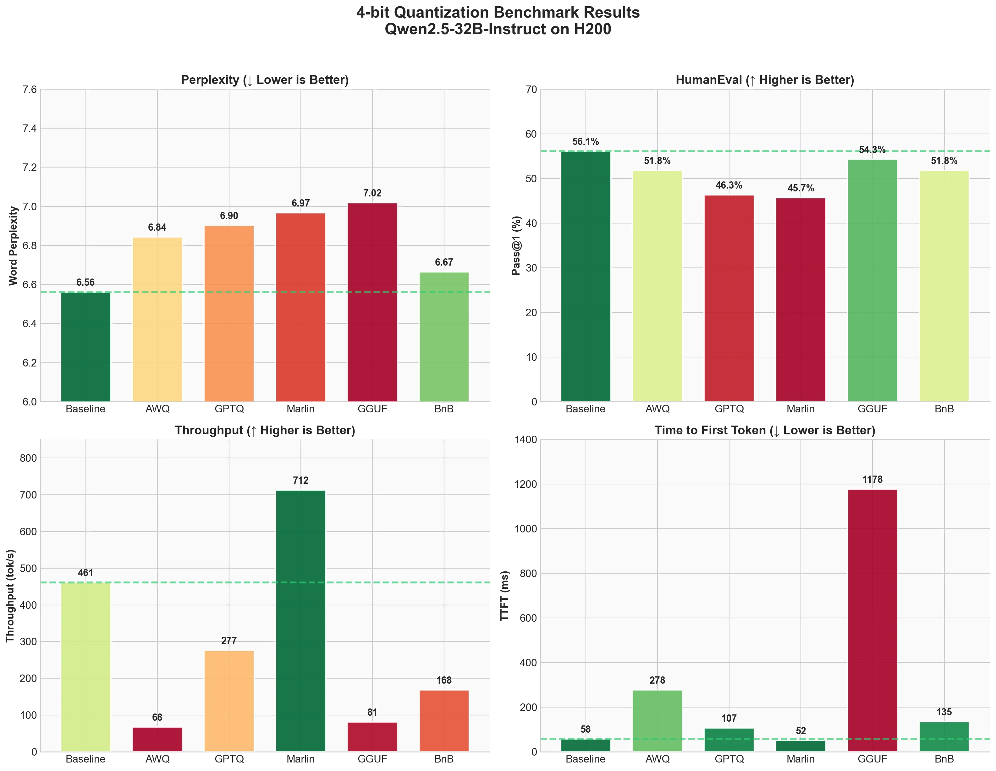
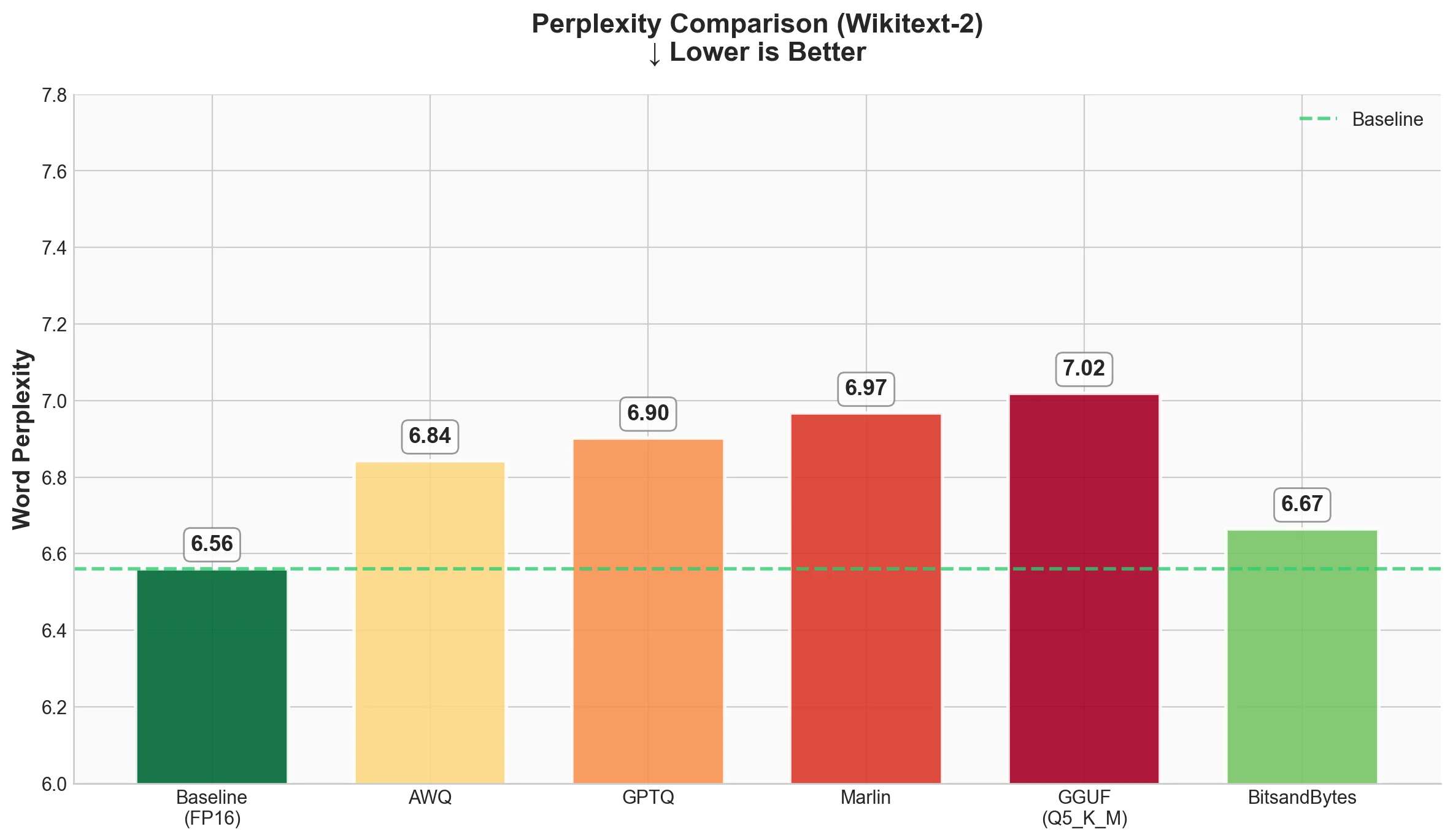
1. Perplexity (Wikitext-2)
Lower perplexity is better. It means the model is less "surprised" by the text and predicts it more accurately.
| Technique | Word Perplexity | Byte Perplexity | Bits per Byte |
|---|---|---|---|
| Baseline (FP16) | 6.5612 | 1.4216 | 0.5075 |
| AWQ | 6.8430 | 1.4328 | 0.5189 |
| GPTQ | 6.9026 | 1.4352 | 0.5212 |
| Marlin-GPTQ | 6.9674 | 1.4377 | 0.5237 |
| Marlin-AWQ | 6.8423 | 1.4328 | 0.5188 |
| GGUF (Q4_K_M) | 6.7376 | 1.4287 | 0.5147 |
| BitsandBytes | 6.6652 | 1.4258 | 0.5118 |
What we see
- All quantized models show slightly higher perplexity than baseline, which is expected.
- BitsandBytes has the smallest quality drop (6.66 vs 6.56 baseline). This is interesting because it doesn't need a pre-quantized checkpoint.
- GGUF (Q4_K_M) comes second with 6.74, showing excellent quality preservation despite being 4-bit.
- AWQ and Marlin-AWQ are nearly identical (6.84 and 6.84), showing that the Marlin kernel preserves AWQ quality while dramatically improving speed.
- GPTQ and Marlin-GPTQ are very close (6.90 and 6.97). The small difference is likely due to numerical precision in the kernel.
The good news: all methods stay within ~6% of baseline perplexity. For most applications, this difference won't be noticeable.
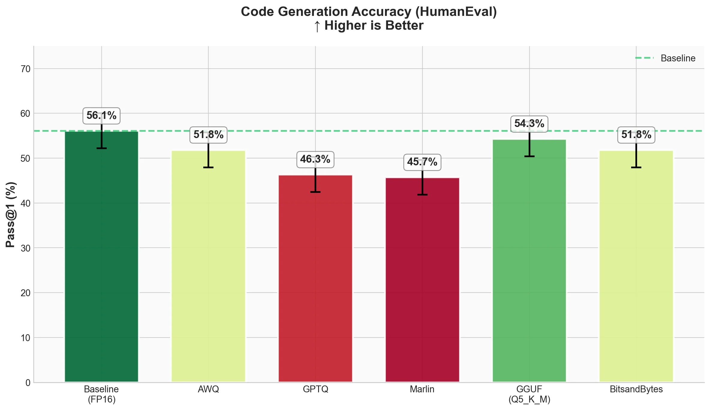
2. Code Generation (HumanEval)
Pass@1 measures what percentage of coding problems the model solves correctly on the first try. Higher is better.
| Technique | Pass@1 | Std Error |
|---|---|---|
| Baseline (FP16) | 0.561 | 0.0389 |
| AWQ | 0.5183 | 0.0391 |
| GPTQ | 0.4634 | 0.0391 |
| Marlin-GPTQ | 0.4573 | 0.039 |
| Marlin-AWQ | 0.5183 | 0.0391 |
| GGUF (Q4_K_M) | 0.5183 | 0.0391 |
| BitsandBytes | 0.5183 | 0.0391 |
What we see
- Baseline solves 56.1% of problems correctly.
- AWQ, Marlin-AWQ, GGUF (Q4_K_M), and BitsandBytes all achieve 51.83%, about 4% below baseline. This consistency shows these methods preserve code generation ability well.
- Notably, Marlin-AWQ matches AWQ's quality while being much faster.
- GPTQ and Marlin-GPTQ drop more significantly to around 46%, which is about 10% below baseline.
This is an interesting finding. GGUF Q4_K_M shows strong code generation despite using a simpler quantization approach (standard scale and zero-point rather than activation-aware or Hessian-based methods), matching AWQ and BitsandBytes performance.
3. Inference Speed (ShareGPT)
Now the fun part - how fast do these methods run? We measured throughput, time to first token (TTFT), and inter-token latency (ITL).
Throughput
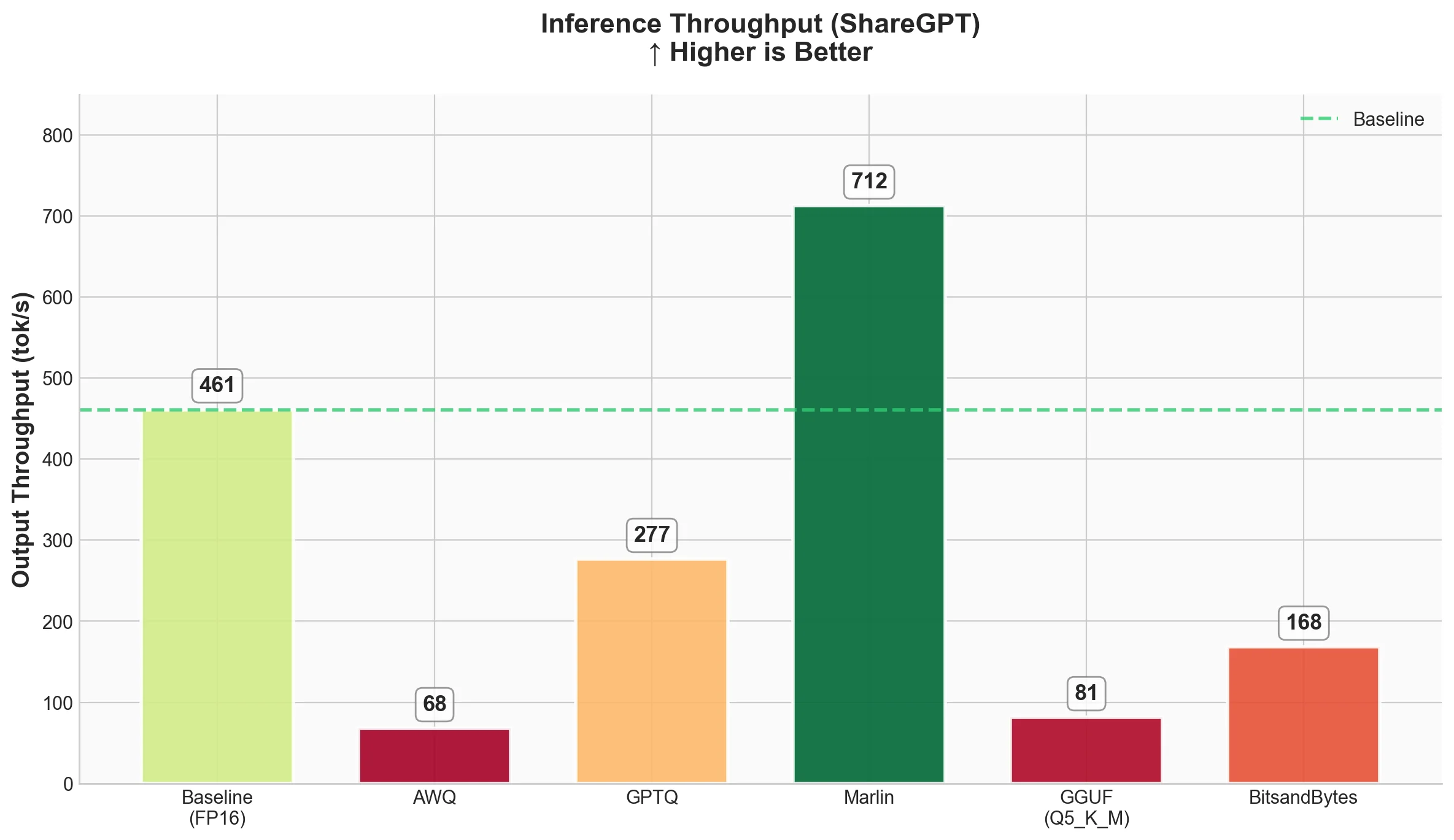
Latency
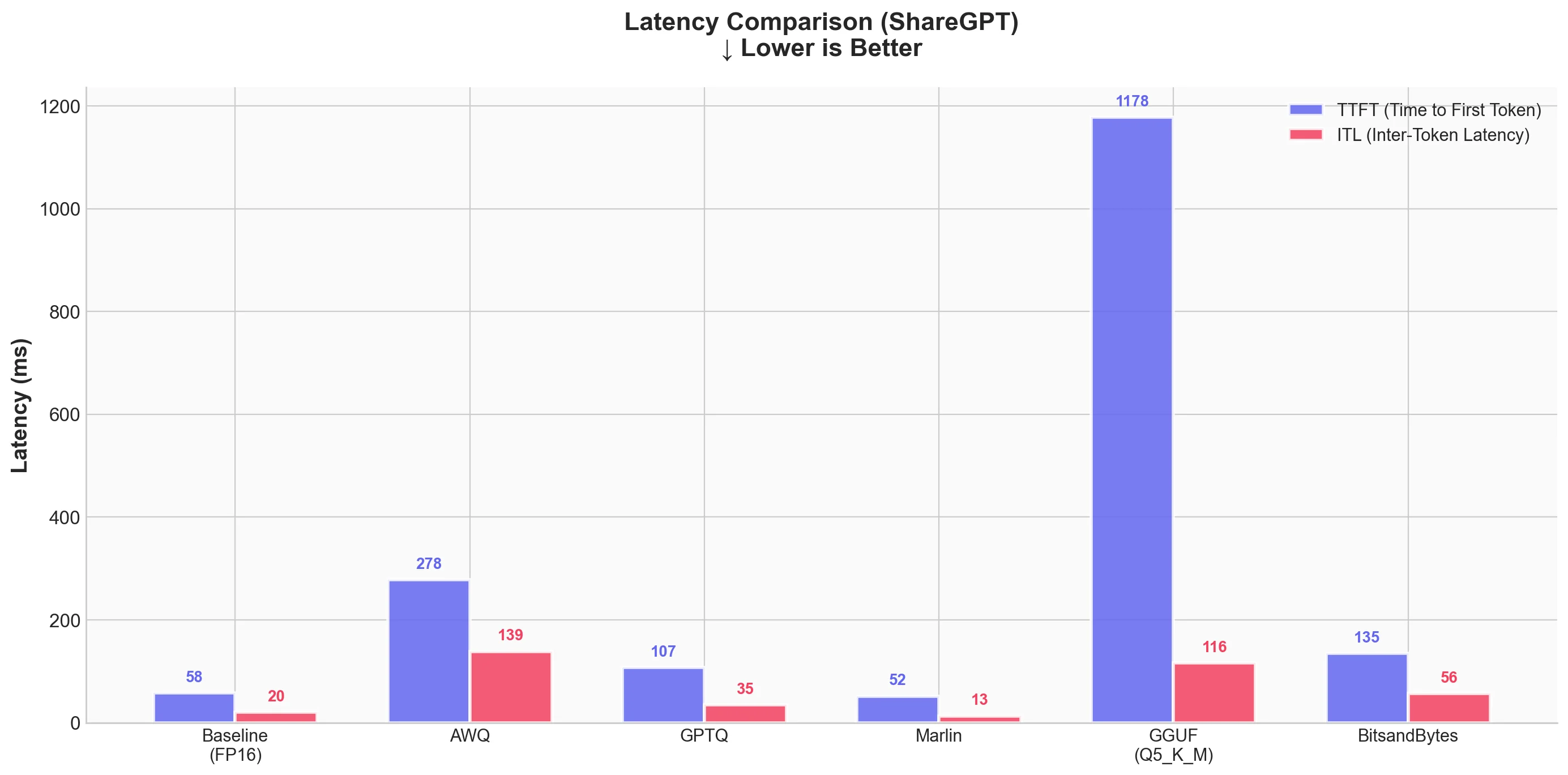
| Technique | Output Throughput (tok/s) | Total Throughput (tok/s) | Mean TTFT (ms) | Mean ITL (ms) |
|---|---|---|---|---|
| Baseline (FP16) | 461.04 | 898.04 | 57.66 | 20.37 |
| AWQ | 67.73 | 132.02 | 277.83 | 138.67 |
| GPTQ | 276.60 | 539.44 | 107.12 | 35.04 |
| Marlin-GPTQ | 712.45 | 1387.80 | 51.90 | 13.11 |
| Marlin-AWQ | 741.04 | 1444.29 | 73.47 | 12.60 |
| GGUF (Q4_K_M) | 93.05 | 179.47 | 957.94 | 101.57 |
| BitsandBytes | 168.37 | 329.34 | 135.31 | 56.50 |
What we see
- Marlin-AWQ is the fastest overall at 741 tok/s output throughput, followed closely by Marlin-GPTQ at 712 tok/s. Both are faster than baseline FP16! This shows the power of optimized kernels.
- Baseline (FP16) is actually quite fast at 461 tok/s output throughput.
- GPTQ without Marlin kernel is slower than baseline (276 tok/s), showing that naive quantized inference doesn't automatically mean faster.
- AWQ without Marlin is surprisingly slow at 67 tok/s. But with Marlin kernel, it achieves 741 tok/s - a 10.9x speedup!
- BitsandBytes runs at 168 tok/s - slower than baseline but reasonable considering it quantizes on-the-fly.
- GGUF runs at 93 tok/s with high TTFT (958ms). The GGUF format has significant overhead in vLLM.
For latency:
- Marlin-AWQ has the best ITL (12.6ms) with good TTFT (73.5ms)
- Marlin-GPTQ has the best TTFT (51.9ms) with excellent ITL (13.1ms)
- Baseline is close with 57.7ms TTFT and 20.4ms ITL
- GGUF has high TTFT at nearly 1 second, which would be noticeable to users
Summary Table
Here's everything in one place
↓ = lower is better, ↑ = higher is better
| Technique | Perplexity ↓ | Pass@1 ↑ | Throughput (tok/s) ↑ | TTFT (ms) ↓ |
|---|---|---|---|---|
| Baseline (FP16) | 6.56 | 56.1% | 461 | 57.7 |
| AWQ | 6.84 | 51.8% | 68 | 277.8 |
| GPTQ | 6.90 | 46.3% | 277 | 107.1 |
| Marlin-GPTQ | 6.97 | 45.7% | 712 | 51.9 |
| Marlin-AWQ | 6.84 | 51.8% | 741 | 73.5 |
| GGUF (Q4_K_M) | 6.74 | 51.8% | 93 | 958.0 |
| BitsandBytes | 6.67 | 51.8% | 168 | 135.3 |
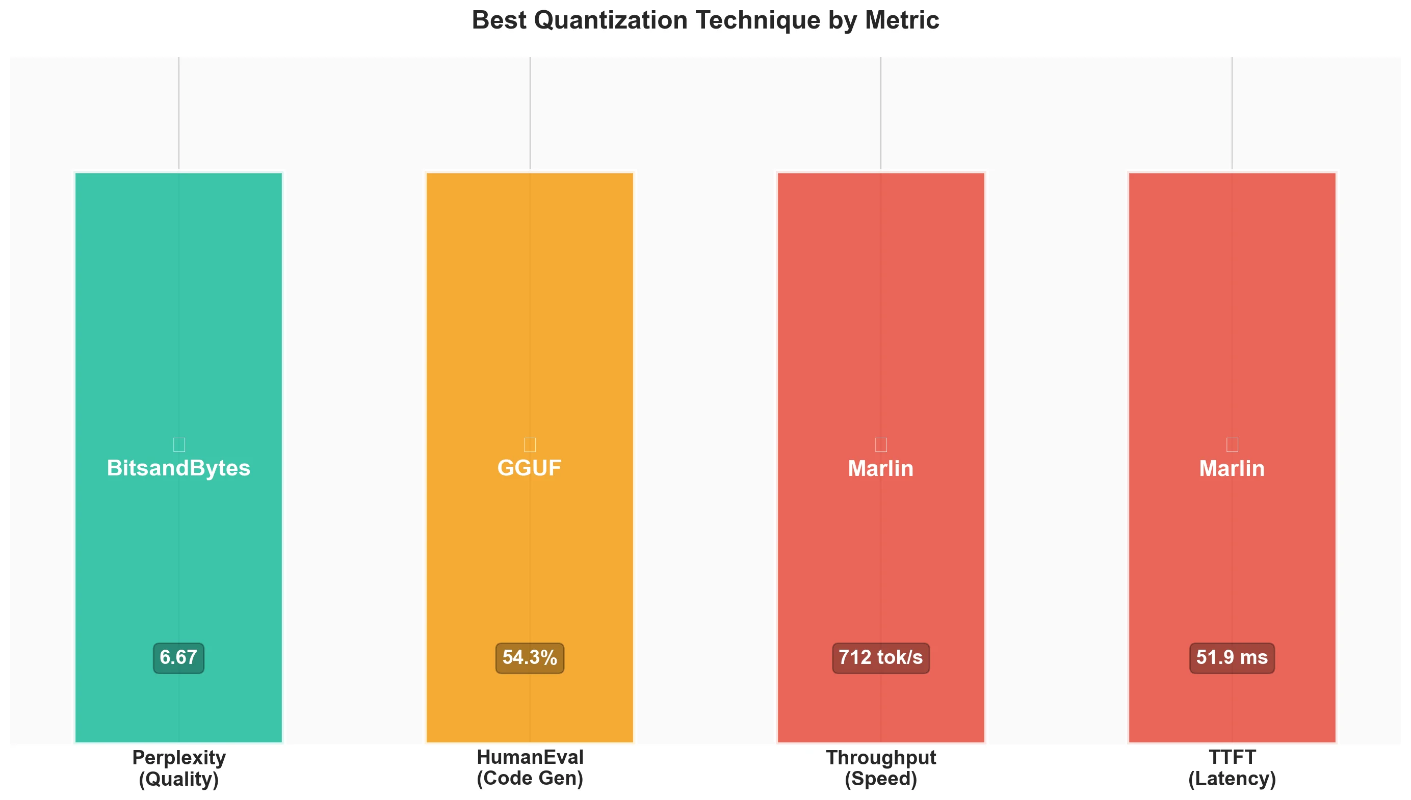
Key Takeaways
-
Quantization works: All methods kept perplexity within ~6% of baseline. 4-bit quantization is practical for real-world use.
-
Kernels matter more than algorithms: Marlin kernels provide massive speedups - 2.6x for GPTQ and 10.9x for AWQ! The quantization algorithm is only half the story.
-
Marlin-AWQ is the sweet spot: It combines AWQ's better quality preservation (51.8% Pass@1) with the fastest throughput (741 tok/s). Best of both worlds.
-
Quality consistency across methods: AWQ, Marlin-AWQ, GGUF (Q4_K_M), and BitsandBytes all achieve the same 51.8% Pass@1 on HumanEval, showing robust code generation preservation.
-
GGUF has overhead in vLLM: While GGUF preserves model quality excellently (6.74 perplexity - second best!), its inference speed in vLLM is poor (93 tok/s). GGUF is better suited for llama.cpp where it was designed to run.
-
Perplexity correlates with code quality: Methods with better perplexity (BitsandBytes at 6.67, GGUF at 6.74) also show strong HumanEval scores (51.8%), confirming that perplexity is a reasonable proxy for model quality.
Ready to start building?
Get a GPU instance running in 90 seconds. JupyterLab, VS Code, or SSH. Per-minute billing so you only pay for what you use.
Try Jarvislabs FreeVerdict
| Your Priority | Best Choice | Runner-up |
|---|---|---|
| Maximum speed | Marlin-AWQ | Marlin-GPTQ |
| Best quality (perplexity) | BitsandBytes | GGUF (Q4_K_M) |
| Code generation | Marlin-AWQ | GGUF / BitsandBytes |
| Speed + Quality | Marlin-AWQ | BitsandBytes |
| Easy setup | BitsandBytes | - |
| Production deployment | Marlin-AWQ | Marlin-GPTQ |
Best for Speed: Marlin-AWQ - Fastest throughput at 741 tok/s (vs 461 tok/s baseline), with excellent ITL (12.6ms). Marlin-GPTQ is close at 712 tok/s with slightly better TTFT.
Best for Quality: BitsandBytes - Lowest perplexity increase (6.67 vs 6.56 baseline), solid HumanEval (51.8%), and no pre-quantized weights needed. GGUF (Q4_K_M) is a close second with 6.74 perplexity.
Best for Speed + Quality: Marlin-AWQ - Combines fastest throughput (741 tok/s) with AWQ's quality preservation (51.8% Pass@1). The sweet spot for production use.
Best for Code Generation: Marlin-AWQ / GGUF / BitsandBytes - All achieve 51.8% Pass@1, tied for best among quantized models. Choose based on your speed requirements.
Our Recommendation: For production, start with Marlin-AWQ. It offers the best combination of speed and quality - faster than Marlin-GPTQ while matching the top HumanEval scores. For experimentation, use BitsandBytes since you don't need pre-quantized models. If using GGUF, consider llama.cpp instead of vLLM for better performance.
Conclusion
We explored 4-bit quantization techniques in vLLM, covering the theory behind each method and running benchmarks on Qwen2.5-32B-Instruct using an H200 GPU.
The bottom line: Marlin-AWQ is the sweet spot - it wins on both speed (741 tok/s) and code generation (51.8% Pass@1), while BitsandBytes offers the best quality preservation (6.67 perplexity). Pick based on your needs, and always benchmark on your actual use case.
Quantization reduces memory per GPU — but when a model is too large even after quantization, you need to split it across multiple GPUs. See our guide on scaling LLM inference with data, pipeline, and tensor parallelism in vLLM for how to do that.
Thanks for reading!
References
Papers
-
AWQ: arXiv:2306.00978
-
GPTQ: arXiv:2210.17323
-
Marlin: arXiv:2408.11743
-
Optimal Brain Surgeon: arXiv:2208.11580
Tools & Libraries
-
BitBLAS: Microsoft TileLang Project. https://github.com/microsoft/BitBLAS
-
BitsandBytes: https://github.com/bitsandbytes-foundation/bitsandbytes
-
llama.cpp (GGUF): https://github.com/ggml-org/llama.cpp
-
TorchAO: PyTorch Architecture Optimization. https://github.com/pytorch/ao
-
lm-evaluation-harness: EleutherAI. https://github.com/EleutherAI/lm-evaluation-harness
-
Apache TVM / TensorIR: https://tvm.apache.org/
Models & Datasets
-
Qwen2.5-32B-Instruct: https://huggingface.co/Qwen/Qwen2.5-32B-Instruct
-
HumanEval: OpenAI. https://github.com/openai/human-eval
-
Wikitext-2: Salesforce. https://huggingface.co/datasets/Salesforce/wikitext
-
ShareGPT: https://huggingface.co/collections/bunnycore/sharegpt-datasets
Documentation & Resources
-
GGUF Format: Hugging Face. https://huggingface.co/docs/hub/en/gguf
-
NVIDIA Hopper Architecture: https://developer.nvidia.com/blog/nvidia-hopper-architecture-in-depth/
-
A Visual Guide to Quantization: Maarten Grootendorst. https://newsletter.maartengrootendorst.com/p/a-visual-guide-to-quantization
-
Introduction to GGML: Hugging Face Blog. https://huggingface.co/blog/introduction-to-ggml
Ready to start building?
Get a GPU instance running in 90 seconds. JupyterLab, VS Code, or SSH. Per-minute billing so you only pay for what you use.
Try Jarvislabs Free