Speculative Decoding in vLLM: Complete Guide to Faster LLM Inference

Introduction

Ever waited for an AI chatbot to finish its answer, watching the text appear word by word slow? It can feel painfully slow, especially when you need a fast response from a powerful Large Language Model (LLM).

The big problem is in how LLMs generate text. They don't just write a paragraph all at once; they follow a strict, word-by-word approach.

1. The model looks at the prompt and the words it has generated so far.
2. It calculates the best next word (token).
3. It adds that word to the text.
4. It repeats the whole process for the next word.

Each step involves complex calculations, meaning the more text you ask for, the longer the wait. For developers building real-time applications (like chatbots, code assistants, or RAG systems), this slowness (high latency) is a major problem.

The Solution: Speculative Decoding

This is where Speculative Decoding steps in!

Instead of waiting for the powerful main model (the target model) to generate one word at a time, we use a small, fast helper (the Draft Model) to guess several words ahead. The main model then only needs to check (verify) those guessed words in a single, super-fast step, much like a quick check.

This lets us skip many slow, sequential steps, resulting in significantly faster text generation and a much better user experience! The great news is that the vLLM framework makes it easy to try out several powerful flavors of this technique. In this blog post, we are going to look at all the available speculative decoding techniques in vLLM. We will study them theoretically first and then use them on two datasets to check how they make a difference in making LLMs fast at generating text.

---

Speculative Decoding Techniques in vLLM

Draft Model Speculative Decoding

Speculative decoding is a collaboration between two models. It allows us to generate text much faster than a massive model could ever do on its own.

1. The target model (Main Model): This is your powerhouse (e.g., Llama-3.3-70B). It provides high-quality, reliable output, but it's slow and expensive to run. Its job is to ensure correctness.
2. The draft model (Helper Model): This is a smaller, lightweight model (e.g., Llama-3.1-8B). It generates text very fast, but it's prone to making small mistakes. Its job is to make "best guesses" to save time.

Crucial Requirement for Speed: For this technique to work efficiently, the draft model and the target model models must share the same model family and, most importantly, the same vocabulary size (i.e., use the same tokenizer). This is vital because the draft model needs to generate tokens that the target model can quickly and directly check without needing costly translation or mapping between different token sets.

The Workflow: Guess, Check, and Keep

The key insight behind speculative decoding is this: while LLMs must generate tokens one by one (each new token depends on the previous), they can verify multiple tokens in parallel. This is because transformer architectures process entire sequences in a single forward pass. So instead of running the expensive target model N times to generate N tokens, we run it just once to verify N guessed tokens simultaneously.

Here is the step-by-step process:

1. Drafting (The Guess): The small draft model quickly reads the context and proposes a short sequence of potential future tokens (let's say, 5 tokens).
2. Verification (The Check): The big target model takes the original input plus those 5 guessed tokens. It runs a single calculation to check them all at once.
3. The Decision (Rejection Sampling): The target model compares its own predictions against the draft model's guesses to decide what to keep. (See "The Logic" below).
4. Correction: As soon as a bad token is found, we discard it and everything after it. The target model inserts the correct token, and the draft model starts guessing again from that new point.

The Logic: How We Decide to Keep or Remove

You might wonder: How exactly does the target model decide if the draft model's guess is "good enough"?

It’s not always about an exact match. We use a probabilistic method called Rejection Sampling.

When the draft model guesses a token, it does so with a certain confidence (probability). The target model then calculates its own probability for that same token. We compare them token-by-token:

• ($P_{target model} \ge P_{draft model}$): If the target model thinks the token is more likely (or equally likely) than the draft model thought, we accept it immediately. The guess was valid.
• ($P_{target model} < P_{draft model}$): If the target model thinks the token is less likely than the draft model did, we don't automatically reject it. Instead, we roll a probability die. The lower the target model's confidence compared to the draft model's, the higher the chance we reject it.

This ensures that the final output distribution mathematically matches the high-quality Main Model, even though a "dumber" model wrote the draft.

A Practical Example: The Workflow in Action

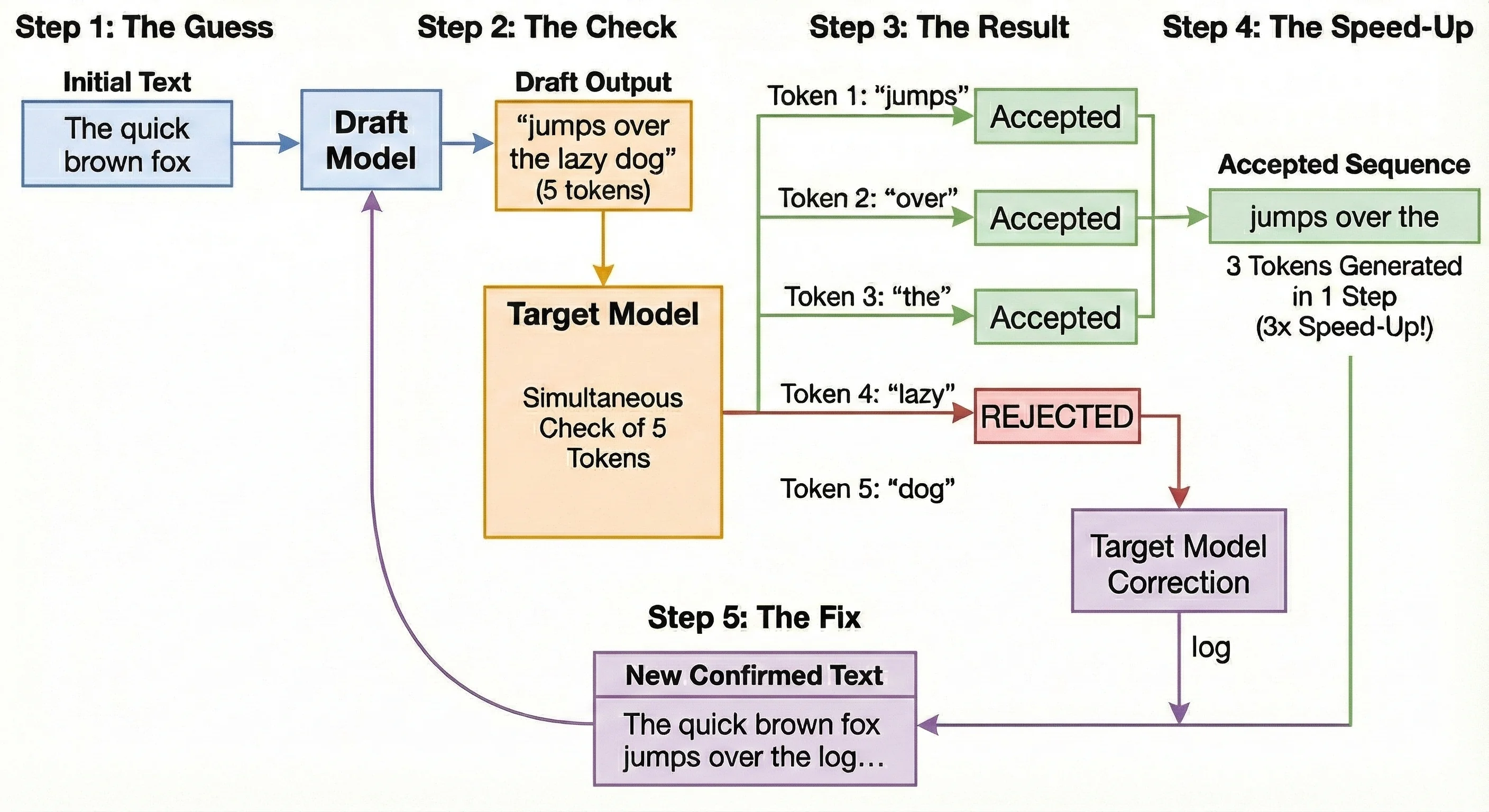
Let's illustrate the speed-up using the classic phrase: "The quick brown fox"

Source : Generated by nano banana pro

Step 1: The Guess

• Action: The fast draft model looks at "The quick brown fox" and predicts 5 new tokens.
• Output: It guesses: "jumps over the lazy dog" (Note: The correct phrase should be "jumps over the log".)

Step 2: The Check

• Action: The powerful target model takes the text and the 5 guesses. It runs one single check to validate all of them simultaneously.

Step 3: The Result

• Action: The target model reviews the probabilities:
  • "jumps": Accepted.
  • "over": Accepted.
  • "the": Accepted.
  • "lazy": REJECTED. The target model calculated that "log" was the probable word here, and the probability for "lazy" was too low to pass the rejection check.

Step 4: The Speed-Up

• Outcome: Even though we failed on the 4th token, we successfully generated 3 tokens ("jumps over the") in the time it usually takes to generate just one. That is a 3x speed-up for this step!

Step 5: The Fix

• Action: The target model replaces the rejected word "lazy" with the correct word: "log".
• Next Round: The system now restarts the drafting process from the new, confirmed text: "The quick brown fox jumps over the log..."

---

N-Gram Matching

N-Gram Matching is a simple yet incredibly effective speculation technique that looks for patterns in the text you've already generated or the input prompt.

How It Works

Unlike a Draft Model that predicts the future, N-Gram Matching looks to the past.

1. Define the Pattern: An N-gram is just a sequence of $N$ tokens. For example, in the phrase "the quick brown fox," a 3-gram would be "quick brown fox."

2. Look Backward: The system takes the last N tokens just generated and searches backward through the prompt and all previously generated text to find where that exact sequence appeared before.

3. Speculate: If a match is found, the system looks at what tokens came immediately after that earlier occurrence. It predicts those same tokens will follow now. For example, if "the quick brown" appeared earlier followed by "fox jumps over," then seeing "the quick brown" again means we can speculate "fox jumps over" as the next tokens.

4. Verify: The target model then verifies these guessed tokens in a single forward pass, just like in draft model speculative decoding.

Why This Is Powerful

This technique shines in contexts where text is often repetitive, such as:

• Code Generation: Repeating boilerplate, loops, or import statements.
• RAG (Retrieval Augmented Generation): Copying large blocks of text exactly as it appears from a source document.

It has the massive advantage of zero VRAM overhead, as it doesn't require loading a second Draft Model!

---

Suffix Decoding

Suffix Decoding is a sophisticated, model-free acceleration technique designed for repetitive workloads like agentic loops and code generation. Instead of a memory-intensive Draft Model, it exploits patterns found in historical text, running entirely on the CPU. This makes it ideal for maximizing speed without adding GPU memory overhead. This technique is conceptually similar to N-gram matching—we pick some recently generated tokens and search for them in the past. The difference is in how we search. N-gram matching performs a linear scan through the prompt and generated text. Suffix Decoding, in contrast, uses pre-built tree data structures that allow for much faster pattern lookups, especially as the text history grows.

The Dual Suffix Tree Cache and Pattern Matching

The core is the highly efficient Suffix Tree data structure, which stores historical patterns from two sources:

Tree Type	Source of Patterns	Purpose in Speculation
Per-Request Tree (Local)	The current prompt and tokens generated so far in the request.	Captures immediate, self-repeating patterns within the ongoing conversation.
Global Tree	Outputs from all previous requests processed by the vLLM service over time.	Provides deep statistical knowledge of common LLM outputs, essential for agentic repetition.

Theoretical Explanation: The Search Mechanism

At each step, SuffixDecoding looks for long, matching patterns ($x_{t-p+1:t}$) to use for speculation.

1. Ongoing Sequence ($x_{1:t}$): This is the full text generated up to the current token $t$.
2. Pattern Length ($p$): This is the size of the recent sequence we are searching for.
3. Pattern Sequence ($x_{t-p+1:t}$): The last $p$ tokens of the ongoing request.

The system attempts to match this pattern by "walking" down the Dual Suffix Trees. If the pattern is found, the system arrives at a node, $N_p$, where all descending paths are the possible continuations of the pattern.

The Scoring and Greedy Expansion

Checking every single possible future sequence is computationally expensive. Suffix Decoding takes a smarter, faster approach using a Greedy Expansion strategy.

Instead of looking at everything, it builds a focused "Speculation Tree"—a roadmap of the most likely future tokens. To decide which branches of the tree to grow, the system relies on two simple probability scores:

1. Step Probability ($C(N)$): How likely is this specific token to follow the one before it?
2. Path Confidence ($D(N)$): How likely is the entire sequence (from the root up to this token) to be correct? This is our main filter for decision-making.

How We Calculate Confidence

The math here is straightforward: The confidence in a new token is based on the confidence of the path that led to it.

$$D(N) = D(\text{Parent}) \times C(N)$$

To get the Path Confidence for a new node ($N$), we take the confidence of its Parent node and multiply it by the Step Probability of the new token. If we are at the very start (the root), the confidence is simply $1$ (or 100%).

The "Greedy" Process

Think of this as chasing the most promising lead.

1. Start: Begin at the last matched token ($N_p$).
2. Evaluate: Look at the available next steps and calculate their Path Confidence.
3. Pick the Winner: Add the leaf node with the highest confidence score to our tree.
4. Repeat: Keep adding the "most likely" next step until the tree reaches its maximum allowed size (MAX_SPEC).

This ensures we spend our computing power expanding only the sequences that the model is most likely to actually use.

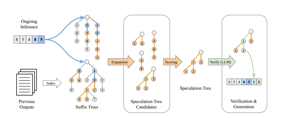
The Visual Workflow

The diagram below illustrates SuffixDecoding's algorithm:

Source : Oliaro, Gabriele, Zhihao Jia, Daniel Campos, and Aurick Qiao. "Suffixdecoding: A model-free approach to speeding up large language model inference." arXiv preprint arXiv:2411.04975 (2024)

This process is broken down into three stages:

Stage 1: Finding Patterns

• Dual Trees: The image shows the current tokens (e.g., 8, 5, 4, 8, 5) being matched against the two Suffix Trees (top for ongoing inference, bottom for previous outputs).
• Expansion: This matching step identifies all possible Speculation Tree Candidates (the sequences in the center-left box) based on the patterns found in the trees.

Stage 2: Building the Speculation Tree

• Scoring & Selection: The system uses the Acceptance Probability ($D(N)$) to score these candidates. It greedily selects the most promising branches, resulting in a single, compact Speculation Tree (the path labeled 1, 2, 3 in the diagram).

Stage 3: Verification and Generation

• Verify: The target model receives the original sequence plus the entire Speculation Tree and performs a single forward pass.
• Accepted Tokens: Tokens are verified in parallel. In the result (box on the right), the target model accepted tokens 1 and 3 (shown in green), which are then added to the final output ($8, 5, 4, 8, 5, 1, 3$). This accelerates generation by accepting multiple tokens in one step.

This entire pattern-matching and drafting process is extremely fast (running on the CPU) and is also adaptive: the number of tokens speculated (MAX_SPEC) is dynamically adjusted based on the pattern match length to avoid wasting computation.

---

MLP Speculators

The MLP Speculator technique builds on the Medusa architecture and was refined by IBM to achieve the high prediction accuracy of a full draft model without the massive memory cost of loading an entire second LLM.

Architecture: The Multi-Headed Lightweight Predictor

Source : Wertheimer, Davis, Joshua Rosenkranz, Thomas Parnell, Sahil Suneja, Pavithra Ranganathan, Raghu Ganti, and Mudhakar Srivatsa. "Accelerating production llms with combined token/embedding speculators." arXiv preprint arXiv:2404.19124 (2024).

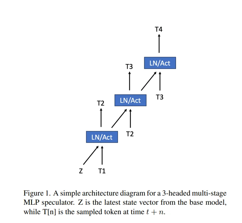
The Speculator is a multi-stage, multi-headed MLP that attaches directly to the target model. Unlike a standard model that predicts just one token, this architecture features distinct "heads" or prediction stages dedicated to looking 1, 2, or 3 steps into the future.

• Attachment & Input: The MLP uses the target model's context embedding vector (internal state Z in above diagram) as its foundation. Crucially, each subsequent head also conditions its prediction on the sampled tokens from the previous head. For example, T2 is predicted using Z and the T1 token generated by the target model.

• Function: Head 1 predicts token T2. Head 2 takes that prediction and predicts token T3, and so on.

Training: The Per-Head Loss Calculation

Source : Wertheimer, Davis, Joshua Rosenkranz, Thomas Parnell, Sahil Suneja, Pavithra Ranganathan, Raghu Ganti, and Mudhakar Srivatsa. "Accelerating production llms with combined token/embedding speculators." arXiv preprint arXiv:2404.19124 (2024).

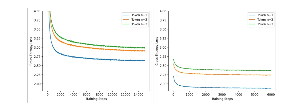
To ensure precise learning, the training process is granular. The target model is frozen, and the MLP is trained using Cross Entropy Loss. However, the system does not just calculate one "lump sum" error. Instead, it calculates three separate losses, one for each speculative step:

1. Step 1 ($Loss_{t+1}$): The error between Head 1's prediction and the actual ground truth for token $t+1$.
2. Step 2 ($Loss_{t+2}$): The error between Head 2's prediction and the actual ground truth for token $t+2$.
3. Step 3 ($Loss_{t+3}$): The error between Head 3's prediction and the actual ground truth for token $t+3$.

Why Separate Curves? The IBM report reveals that these losses behave differently. Predicting the immediate next token ($t+1$) is "easier," so its loss drops quickly. Predicting further out ($t+3$) is harder and relies on the accuracy of the previous steps, resulting in a higher loss curve. By tracking these separately, the training ensures that errors in the immediate future ($t+1$) don't get hidden by errors in the distant future ($t+3$).

The Two-Stage Training Scheme

The training occurs in two distinct phases to maximize stability and accuracy:

1. Stage 1: Input Alignment (Proxy Data): The speculator is trained on standard text data batches with long contexts. Here, it learns to map the target model's embeddings to valid next tokens.
2. Stage 2: Output Alignment (Model Distillation): The training switches to use generated outputs from the target model itself as the ground truth. The loss function now forces the MLP to mimic exactly what the frozen target model would have generated. This aligns the specific "personality" of the MLP to the target model.

How It Works: Inference and Prediction

The MLP Speculator works by rapidly predicting multiple tokens in sequence:

1. Pass 1: Target Model Forward Pass: The target model performs its forward pass, producing the context embedding vector for the current token.
2. Pass 2: Speculator Forward Pass: The MLP Speculator takes that context vector and rapidly generates a sequence of $K$ speculative tokens. The speculator uses the logits from the first predicted token to condition the second prediction, building the sequence $T_{t+1}, T_{t+2}, \dots, T_{t+K}$.
3. Verification: The entire speculated sequence is then bundled and sent to the target model for verification in a single forward pass.

Key Advantages for Production

1. Massive VRAM Savings: Since the MLP is tiny (often ~1/10th the parameters or less), the memory overhead is minimal compared to a full draft model.
2. High Acceptance Rate: By leveraging the target model's own context, the MLP's predictions are highly accurate, accelerating wall-clock inference speeds by a factor of 2-3x.
3. Efficiency: It attaches directly to the target model, avoiding the need for complex, separate model management.

---

EAGLE Technique

The EAGLE (Extrapolation Algorithm for Greater Language-Model Efficiency) family represents a paradigm shift in speculative decoding. While Draft Models require a completely separate LLM (creating memory and tokenizer headaches) and MLP Speculators use simple projections, EAGLE takes a "best of both worlds" approach.

It trains a lightweight draft head (typically just 1-2 transformer layers) that plugs directly into your Target Model. This head reuses the Target Model's internal feature maps to predict tokens, adding minimal parameter overhead (under 5% for 70B models) while delivering massive speedups.

The Evolution: EAGLE 1, 2, and 3

Source : Generated by nano banana pro

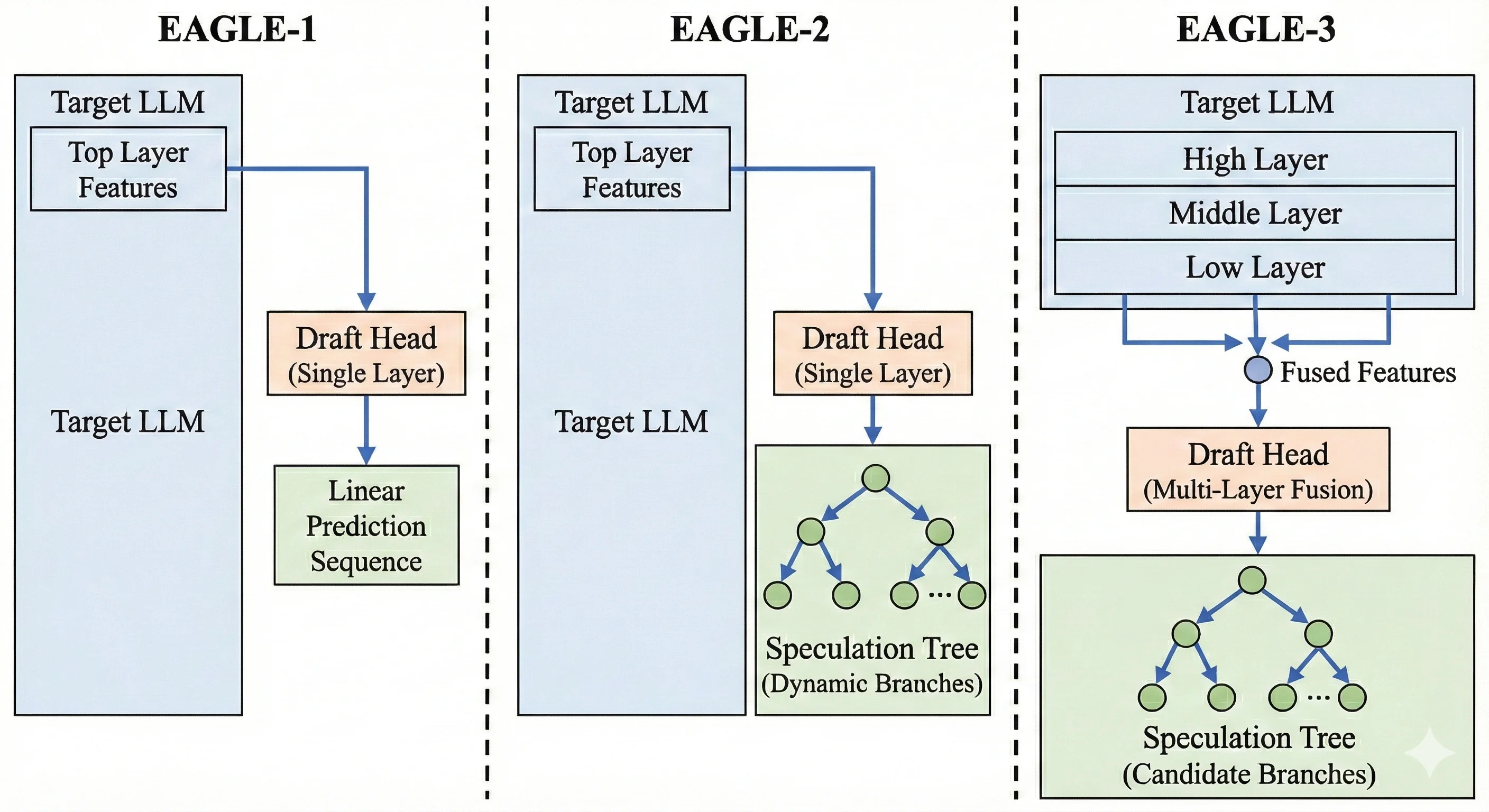
To understand why EAGLE-3 is the current state-of-the-art for speculative decoding, we must look at how the technique evolved:

• EAGLE-1 (The Original): This version introduced the idea of a single-layer draft head reusing the Target Model's top-layer features (the features right before the final output).

  • Limitation: It suffered from "feature uncertainty." It was trained on perfect "ground truth" data but had to generate based on its own noisy predictions during inference. This caused acceptance rates to drop quickly as it predicted further ahead.

• EAGLE-2 (Dynamic Trees): This iteration improved the inference strategy. It introduced dynamic draft trees that contextually adjusted the shape of the speculation tree.

  • Improvement: It became smarter about how to guess (pruning low-confidence branches early), but it still relied on the same fundamental feature extraction as EAGLE-1, limiting its maximum accuracy.

• EAGLE-3 (The Breakthrough): This version fundamentally changes how the draft head learns and what it sees.

  • Key Innovation 1 (Multi-Layer Fusion): Instead of just looking at the top layer, EAGLE-3 extracts and fuses features from the Low, Middle, and High layers of the Target Model. This provides a much richer context for prediction.
  • Key Innovation 2 (Training-Time Test): It solves the "Distribution Mismatch" problem by simulating the noisy inference process during the training phase itself.

Training Strategy: The "Training-Time Test" (TTT)

EAGLE-3's training strategy is its secret weapon. In traditional approaches, draft heads are trained on perfect, "ground truth" inputs. But in the real world, the draft head has to predict Token 3 based on its own guess for Token 2. If its guess for Token 2 was slightly off, it gets confused.

EAGLE-3 uses Training-Time Test (TTT) to fix this:

1. Native Step: The model tries to predict the next token using perfect features from the Target Model.
2. Simulated Steps: Crucially, it then feeds its own predictions back as inputs to predict subsequent tokens.
   • Example: If predicting "How can I help," for the token "help," it uses its own (potentially imperfect) prediction of "I" as input rather than the ground truth.

This forces the draft head to learn how to recover from its own mistakes, keeping the acceptance rate flat (70-80%) even deep into the generated sequence.

Inference Strategy: Tree Attention

During inference, EAGLE-3 does not generate a single line of text. It generates a Candidate Tree.

1. Tree Construction: From the prompt "The weather is", it might predict "sunny" (high probability) and "getting" (lower probability). It then branches out from both.
   • Constraint: It uses confidence-based pruning to stop growing branches that are unlikely to be accepted.
2. Tree Attention Verification: The Target Model verifies all these branches in a single forward pass. It uses a specific Tree Attention Mask so that a token in Branch A doesn't "see" tokens from Branch B.
3. Selection: The valid path is selected, and the rest are discarded.

For a more in-depth understanding, refer to this EAGLE-3 blog post.

---

Benchmark Setup

To move beyond theoretical papers and measure real-world impact, we ran extensive benchmarks in a controlled production environment using vLLM.

Note on Scope: While we discussed five techniques earlier, we are benchmarking only three of them here: N-Gram Matching, Suffix Decoding, and EAGLE (with two variants: EAGLE and EAGLE-3). We also include a Baseline (No Speculation) for comparison.

• Why only three? At the time of writing, Draft Model (separate weights) and MLP Speculator implementations are not fully supported in the stable vLLM version 0.12.0 release we tested. Therefore, we focused on the most reliable methods available today.

The Datasets: Real-World Proxies

ShareGPT (1,000 Prompts)

• What it is: A collection of real-world, multi-turn conversations between humans and ChatGPT. We randomly sampled 1,000 prompts to create a robust test set.
• Why we chose it: This represents the "General Chat" use case.
  • High Variance: Human conversations are messy, creative, and unpredictable.
  • Stress Test: Because the output isn't highly repetitive, this dataset effectively stress-tests a Draft Model's ability to "think" and generalize, rather than just memorize patterns. It is the standard for evaluating general-purpose instruct models.
• How to download:

  wget https://huggingface.co/datasets/anon8231489123/ShareGPT_Vicuna_unfiltered/resolve/main/ShareGPT_V3_unfiltered_cleaned_split.json

SWE-bench Lite (300 Samples)

• What it is: A curated dataset based on real GitHub issues and pull requests from popular Python repositories. It challenges the model to solve actual software engineering problems. We used 300 samples for this benchmark.
• Why we chose it: This represents the "Agentic & Coding" use case.
  • High Structure: Code is inherently repetitive (standard imports, variable names, syntactic structures like loops and classes).
  • Pattern Heavy: This structure theoretically favors pattern-matching techniques (like Suffix Decoding and N-Gram), allowing us to see if they can outperform smarter draft models in specialized, repetitive tasks.
• How to download:
  • Use following script to download this dataset and convert it to vllm compatible format.

  from datasets import load_dataset
  import json
  
  ds = load_dataset("princeton-nlp/SWE-bench_Lite", split="test")
  
  with open("swe_bench_vllm.jsonl", "w") as f:
    for row in ds:
        prompt = f"Repo: {row['repo']}\n\nProblem:\n{row['problem_statement']}\n\nCode Context:\n{row['hints_text']}\n\nPlease generate the patch to fix this issue:\n"
        f.write(json.dumps({"prompt":prompt}) + "\n")

---

Hardware & Models

We tested two distinct classes of models to see how speculative decoding scales from efficient single-GPU deployments to massive enterprise-grade intelligence.

The Hardware

• For 8B Models (The Efficiency Tier)

  • GPU: 1x NVIDIA L40S (48GB VRAM)
  • Why: A single L40S provides massive compute density for smaller models. The 48GB memory easily fits the 8B model weights (~16GB in bf16) while leaving ample room for a large KV cache and batch size.

• For 70B Models (The Performance Tier)

  • GPU: 2x NVIDIA H200 (141GB VRAM each)
  • Why: The Llama-3.3-70B model requires ~140GB just for its weights (in bf16). We utilized two H200s to ensure we weren't bottlenecked by memory capacity, allowing us to test long context lengths and high concurrency without OOM (Out Of Memory) errors.

---

Getting the Hardware

To run these experiments, we used JarvisLabs. Here's how to set up your own instance:

1. Log in to JarvisLabs and navigate to the dashboard.
2. Create an Instance: Click Create and select your desired GPU configuration.
3. Select Your GPU:
   • Choose L40S for the lower-cost option.
   • Choose H200 for higher performance.
4. Choose the Framework: Select PyTorch from the available frameworks.
5. Launch: Click Launch. Your instance will be ready in a few minutes.

---

Experimental Configurations

We benchmarked four distinct setups for each model size. Note that EAGLE and EAGLE 3 requires specific pre-trained checkpoints, while N-Gram and Suffix are purely algorithmic and require no external weights.

Configuration 1: Llama-3.1-8B-Instruct

Technique	Target Model	Speculative Configuration
Baseline (No Spec)	Llama-3.1-8B-Instruct	None (Standard Autoregressive)
N-Gram Matching	Llama-3.1-8B-Instruct	{"method": "ngram", "prompt_lookup_max": 4}
Suffix Decoding	Llama-3.1-8B-Instruct	{"method": "suffix"}
EAGLE	Llama-3.1-8B-Instruct	'{"method":"eagle", "model":"yuhuili/EAGLE-LLaMA3.1-Instruct-8B", "draft_tensor_parallel_size":1, "num_speculative_tokens":2}'
EAGLE 3	Llama-3.1-8B-Instruct	'{"method":"eagle3", "model":"yuhuili/EAGLE3-LLaMA3.1-Instruct-8B", "draft_tensor_parallel_size":1, "num_speculative_tokens":2}'

Configuration 2: Llama-3.3-70B-Instruct

Technique	Target Model	Speculative Configuration
Baseline (No Spec)	Llama-3.3-70B-Instruct	None (Standard Autoregressive)
N-Gram Matching	Llama-3.3-70B-Instruct	{"method": "ngram", "prompt_lookup_max": 4}
Suffix Decoding	Llama-3.3-70B-Instruct	{"method": "suffix"}
EAGLE	Llama-3.3-70B-Instruct	'{"method":"eagle", "model":"RedHatAI/Llama-3.3-70B-Instruct-speculator.eagle3", "draft_tensor_parallel_size":1, "num_speculative_tokens":2}'
EAGLE 3	Llama-3.3-70B-Instruct	{"method":"eagle3", "model":"RedHatAI/Llama-3.3-70B-Instruct-speculator.eagle3", "draft_tensor_parallel_size":1, "num_speculative_tokens":2}

---

Benchmarking Methodology

To accurately simulate a production environment, we adopted a robust Client-Server architecture using vLLM's built-in benchmarking tools. This ensures we capture the full system latency, including HTTP overhead and the scheduler's behavior under load.

Step 1: Launch the vLLM Server

First, we spin up the model in online mode using vllm serve. This acts as the API endpoint.

We used the following base command for all experiments. The key variable is the --speculative-config argument, which we swapped out for each technique.

For Llama-3.1-8B (Single L40S)

vllm serve meta-llama/Llama-3.1-8B-Instruct \
  --dtype bfloat16 \
  --seed 42 \
  --tensor-parallel-size 1 \
  --gpu_memory_utilization 0.8 \
  --speculative-config <INSERT_CONFIG_STRING_HERE>

For Llama-3.3-70B (Dual H200s) The 70B model is too large for a single GPU. We used Tensor Parallelism (TP=2) to split it across two H200s. Note the higher memory utilization to maximize the context window.

vllm serve meta-llama/Llama-3.3-70B-Instruct \
  --dtype bfloat16 \
  --seed 42 \
  --tensor-parallel-size 2 \
  --gpu_memory_utilization 0.9 \
  --speculative-config <INSERT_CONFIG_STRING_HERE>

---

The 4 Configurations We Tested Replace <INSERT_CONFIG_STRING_HERE> with the specific JSON string for the technique you are testing:

Technique	Configuration String
Baseline	--speculative-config (Remove the argument entirely)
N-Gram	'{"method": "ngram", "num_speculative_tokens": 5, "prompt_lookup_max": 4}'
Suffix	'{"method": "suffix"}'
EAGLE	'{"method": "eagle", "model": "yuhuili/EAGLE-LLaMA3.1-Instruct-8B", "num_speculative_tokens": 2, "draft_tensor_parallel_size": 1}'
EAGLE 3	'{"method": "eagle3", "model": "yuhuili/EAGLE3-LLaMA3.1-Instruct-8B", "num_speculative_tokens": 2, "draft_tensor_parallel_size": 1}'

Step 2: Stress Test with the Benchmarking Client

Once the server was running (on http://127.0.0.1:8000), we used vLLM's built-in benchmarking tool, vllm bench serve, to stress test it. This command acts as a load-testing client—it fires requests at the server and measures key metrics like throughput, latency, and time-per-token under realistic serving conditions.

We tested two different scenarios:

Scenario A: General Chat (ShareGPT) This command sends 1,000 diverse prompts to the server.

vllm bench serve \
  --model meta-llama/Llama-3.1-8B-Instruct \
  --dataset-name sharegpt \
  --dataset-path ./ShareGPT_V3_unfiltered_cleaned_split.json \
  --host 127.0.0.1 \
  --port 8000 \
  --request-rate inf \
  --max-concurrency 10 \
  --seed 42

Scenario B: Coding Tasks (SWE-bench-lite) For the coding benchmark, we used a custom dataset adapter and used test set which is of 300 samples.

vllm bench serve \
  --model meta-llama/Llama-3.1-8B-Instruct \
  --dataset-name custom \
  --dataset-path swe_bench_vllm.jsonl \
  --host 127.0.0.1 \
  --port 8000 \
  --request-rate inf \
  --max-concurrency 10 \
  --seed 42 \
  --num-prompts 300

---

Results & Analysis

The benchmarks reveal a fascinating story. The winner depends entirely on your model size and, more importantly, your specific workload (Chat vs. Code).

Experiment A: Llama-3.1-8B (The Efficiency Tier)

We ran the 8B model on a single L40S GPU. This setup represents the most common deployment for cost-efficient microservices and edge cases.

Unlike larger models, the 8B model is compute-bound rather than memory-bound. The model weights fit comfortably in GPU memory, so the bottleneck shifts to how fast the GPU can perform the actual matrix multiplications. This means the target model itself is already quite fast, and speculative decoding techniques need to have very low overhead to provide meaningful speedups—any extra computation from the draft model directly competes with the target model for GPU cycles.

Scenario 1: General Chat (ShareGPT)

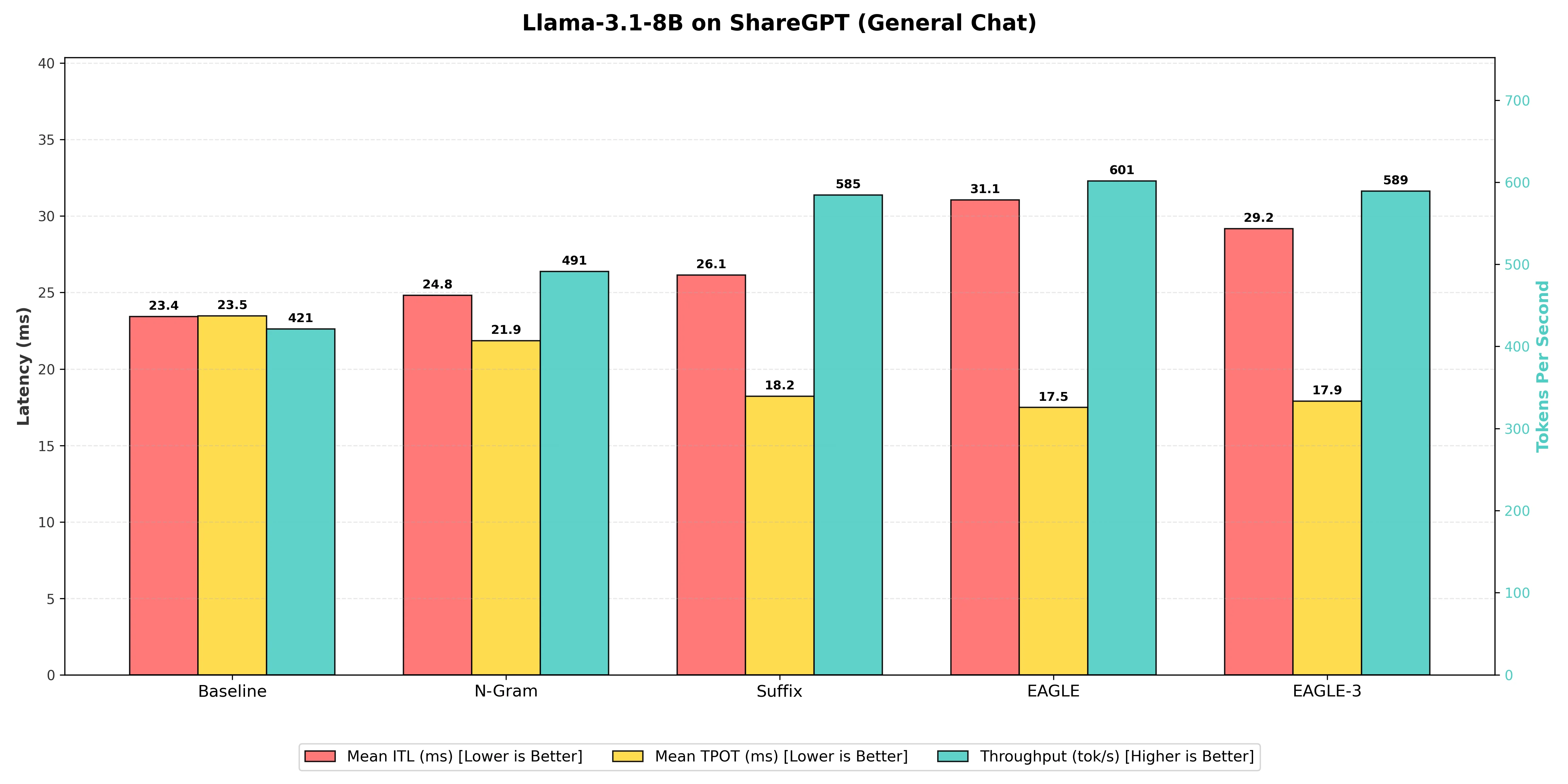
In open-ended conversations, the EAGLE techniques (v1 and v3) proved superior. Because human conversation is unpredictable, simple pattern matching (like looking at previous words) struggles to look far ahead. EAGLE uses a learned "draft head" a tiny, smart component that understands context allowing it to accurately predict 2-3 tokens at a time.

Benchmarking Table

Decoding Technique	Output Token Throughput (tok/s)	Mean Time Per Output Token (ms)	Mean Inter Token Latency (ms)	Speedup Ratio (vs. Baseline)
N-gram Matching	491	21.85	24.8	1.17x
Suffix Decoding	585	18.21	26.1	1.39x
EAGLE-3	589	17.90	29.2	1.40x
EAGLE (Winner)	601	17.49	31.1	1.43x

• EAGLE Technique: On the 8B model, the standard EAGLE technique achieved the highest output throughput at 601 tokens per second, resulting in a 1.43x speedup over the Baseline. This demonstrates its superiority in complex, open-ended chat generation by leveraging the model's internal features for smarter token prediction. EAGLE takes slightly more time to process each individual step (higher Inter-Token Latency of 31.1ms vs 23.4ms baseline) because it predicts and verifies multiple tokens at once. However, this trade-off is highly favorable: by generating text in efficient "chunks" rather than word-by-word, the overall speed of writing the full response is significantly faster.

• Suffix Decoding: With 585 tokens per second, Suffix Decoding was effective for general chat, providing a 1.39x speedup. It was only 2.7 % slower than EAGLE on the 8B model, challenging the assumption that it is only useful for repetitive coding tasks. Its lower overhead compared to EAGLE makes it a very strong "plug-and-play" contender that requires no training.

• N-gram Matching: The N-gram matching method showed the lowest performance gain among the speculative techniques, reaching 491 tokens per second. While it offers a 1.17x speedup over the Baseline, it was substantially 18.3% slower than the leading EAGLE technique, indicating its limitations in capturing the less repetitive patterns of natural conversation.

• Baseline (Vanilla Decoding): The standard one-token-at-a-time generation provided the slowest raw speed at 421 tokens per second, establishing the necessary benchmark for assessing the effectiveness of all speed-up methods.

Scenario 2: Coding Tasks (SWE-bench-lite)

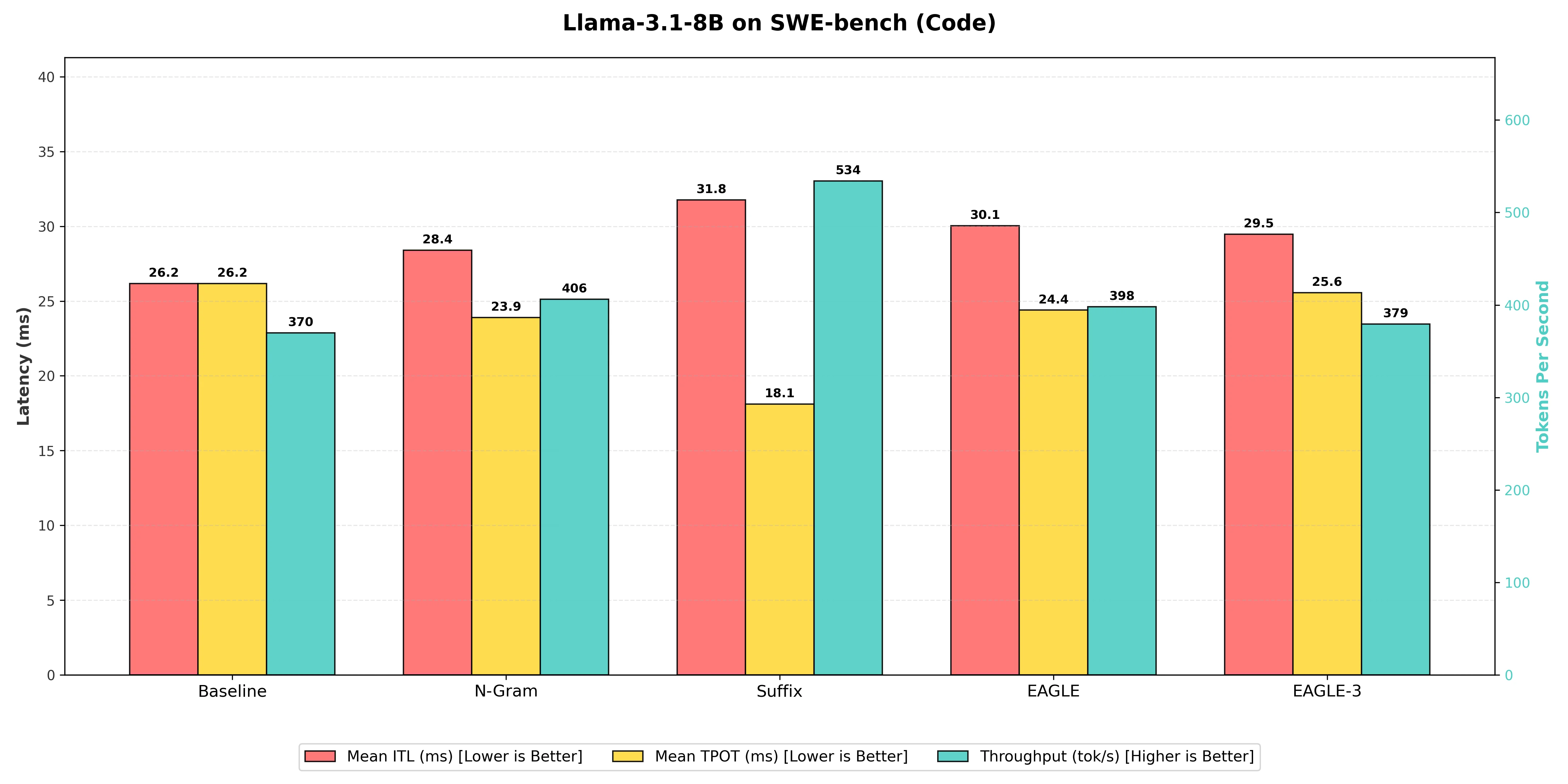
Here, the leaderboard flipped completely compared to the general chat scenario. Code is highly structured. It repeats variable names, indentation patterns, and boilerplate imports constantly, which changes which speculative method works best.

Benchmarking Table

Decoding Technique	Output Token Throughput (tok/s)	Mean Time Per Output Token (ms)	Mean Inter Token Latency (ms)	Speedup Ratio (vs. Baseline)
N-gram Matching	406	23.90	28.4	1.10x
EAGLE	398	24.40	30.0	1.08x
EAGLE-3	379	25.56	29.5	1.03x
Suffix Decoding (Winner)	534	18.10	31.8	1.45x

• Suffix Decoding: On the 8B model, Suffix Decoding achieved a good lead with 534 tokens per second, a 1.45x speedup over the Baseline at 370 tok/s. This method is explicitly designed to thrive in the repetitive, structured environment of code and agentic loops, maximizing its acceptance rate by matching long patterns from the prompt and previous outputs.

• N-gram Matching: Performed decently on this task due to code's repetitive nature, reaching 406 tokens per second, giving it a 1.10x speedup over the Baseline. However, it was 24.0% slower than the Suffix Decoding technique, which captures longer-range patterns more effectively.

• EAGLE & EAGLE-3: Surprisingly, on the 8B model, both EAGLE variants struggled to match the efficiency of Suffix Decoding. Standard EAGLE reached 398 tok/s (1.08x speedup), while EAGLE-3 actually performed slightly worse at 379 tok/s (1.03x speedup), barely beating the baseline. This confirms that for smaller models on rigid tasks, simple heuristic matching (Suffix) often beats complex trained predictors. This is likely because the overhead of the EAGLE draft model outweighs its benefits when the target model is already fast or the task is highly predictable.

• Baseline (Vanilla Decoding): The standard one-token-at-a-time generation provided the slowest raw speed at 370 tokens per second, confirming that any predictive method provides a significant speedup for coding tasks, but the type of method matters immensely depending on your model size.

Experiment B: Llama-3.3-70B (The Scale Tier)

Running on 2x H200s, the 70B model showed us that memory bandwidth how fast we can move data between the GPU memory and the compute units is the ultimate bottleneck.

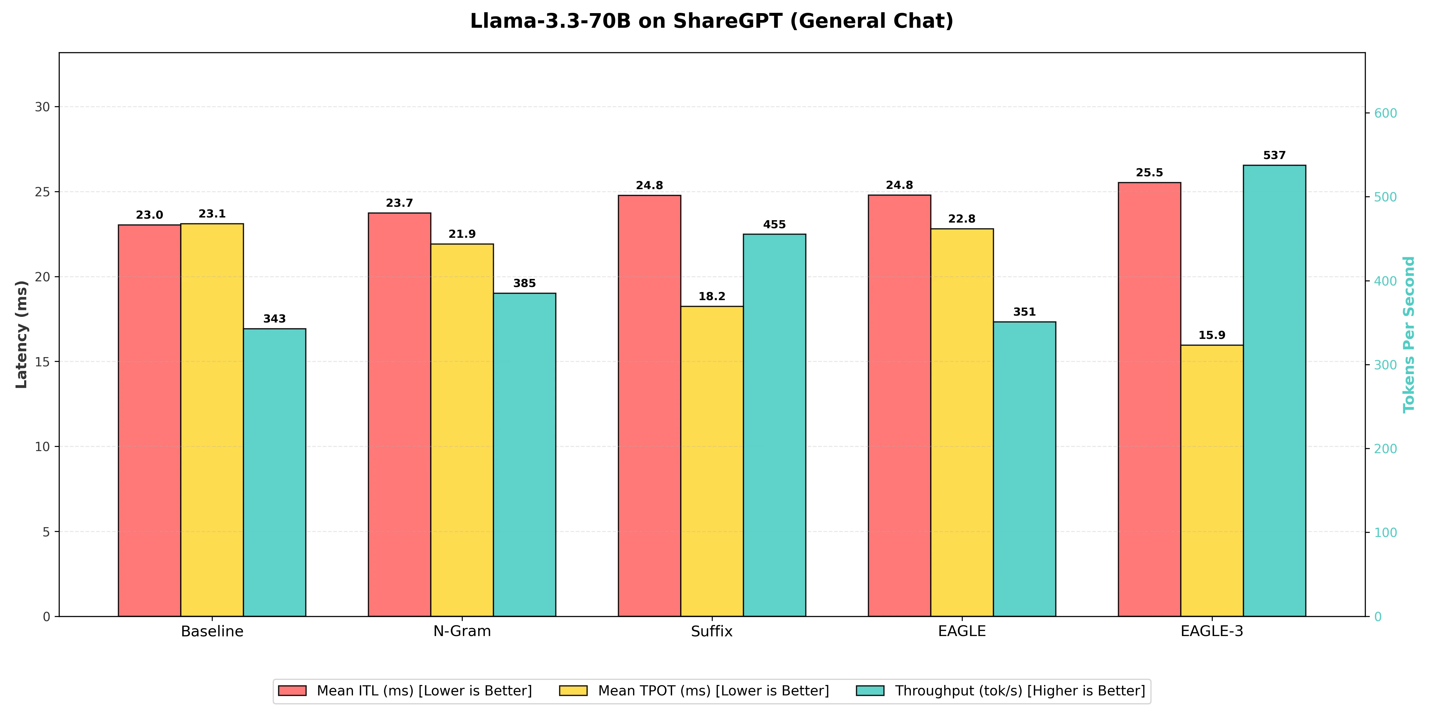
Scenario 1: General Chat (ShareGPT)

For massive models like Llama-3.3-70B, running on dual H200 GPUs, every single step and memory access is expensive. This is where the efficiency of the speculative decoding method becomes critical. When serving LLMs, inference is often memory-bound, meaning the time spent moving data (weights) is the biggest bottleneck, and a larger model makes this worse.

This is where the EAGLE-3 technique truly shines. While the standard EAGLE implementation struggled to gain traction on this specific setup, EAGLE-3 uses a more advanced, lightweight draft head to predict the next few tokens with much higher accuracy. This significantly reduces the number of times the heavy 70B model needs to be fully accessed.

To clearly see the advantage of the more intelligent EAGLE-3 approach on this massive model, we use the Baseline's Output Token Throughput of 343 tokens per second to calculate all speedups:

Benchmarking Table

Decoding Technique	Output Token Throughput (tok/s)	Mean Time Per Output Token (ms)	Mean Inter Token Latency (ms)	Speedup Ratio (vs. Baseline)
EAGLE (Standard)	351	22.81	24.8	1.02x
N-gram Matching	385	21.90	23.7	1.12x
Suffix Decoding	455	18.24	24.8	1.33x
EAGLE-3 (Winner)	537	15.95	25.5	1.57x

• EAGLE-3: The EAGLE-3 technique was the winner, delivering a throughput of 537 tokens per second. This resulted in a 1.57x speedup over the Baseline. It outperformed the standard EAGLE implementation, proving that its improved draft head architecture is essential for scaling to 70B models effectively.

• Suffix Decoding: This method achieved a very respectable 455 tokens per second, a strong 1.33x speedup over the Baseline. While it was 15.3% slower than EAGLE-3, it remains a robust choice because it requires no extra training or draft model management, offering a "free" performance boost.

• N-gram Matching: The basic pattern matching of N-gram showed a modest uplift, reaching 385 tokens per second (1.12x speedup). On this larger model, the simple statistical prediction methods struggled to keep up with the advanced lookahead capabilities of EAGLE-3.

• EAGLE (Standard): Surprisingly, the standard EAGLE implementation barely outperformed the baseline, reaching only 351 tokens per second (1.02x speedup). This highlights a critical finding: for the Llama-3.3-70B architecture, upgrading to EAGLE-3 is mandatory to see real gains.

• Baseline (Vanilla Decoding): The standard generation provided the slowest raw speed at 343 tokens per second. The gap between this and EAGLE-3 (nearly 200 tokens/second difference) illustrates just how much GPU potential is left on the table without speculative decoding.

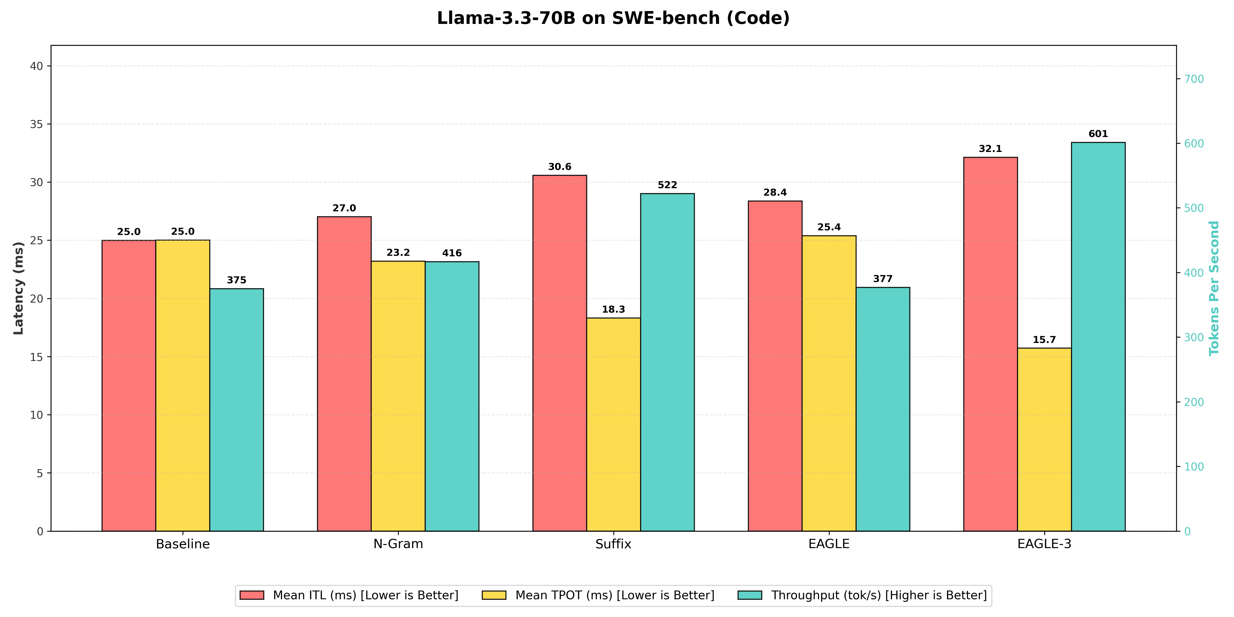
Scenario 2: Coding & Agents (SWE-bench-lite)

This is where we expected the leaderboard to flip back to Suffix Decoding (as it did with the 8B model). In "Agentic" workflows, where the model often reads its own previous outputs (loops), text repetition is incredibly high, which usually favors pattern matching.

However, the results for the 70B model told a different story. While Suffix Decoding performed admirably, EAGLE-3—being the current state-of-the-art for speculative decoding—proved efficient enough to maintain its lead even in this structured domain.

For this code-heavy task, the Baseline throughput was approximately 375 tokens per second.

Benchmarking Table

Decoding Technique	Output Token Throughput (tok/s)	Mean Time Per Output Token (ms)	Mean Inter Token Latency (ms)	Speedup Ratio (vs. Baseline)
EAGLE (Standard)	377	25.38	28.4	1.01x
N-gram Matching	416	23.20	27.0	1.11x
Suffix Decoding	522	18.32	30.6	1.39x
EAGLE-3 (Winner)	601	15.73	32.1	1.60x

• EAGLE-3: As expected from the current state-of-the-art, EAGLE-3 achieved the highest throughput at 601 tokens per second, resulting in a 1.60x speedup over the Baseline. Unlike the smaller 8B model where Suffix won this category, the 70B EAGLE-3 draft model is robust enough to predict structured code patterns more effectively than even the best heuristic methods.

• Suffix Decoding: Achieved a strong 522 tokens per second, resulting in a 1.39x speedup over the Baseline. While it didn't take the top spot, it remains a highly competitive option. It outperformed N-gram matching by 25.5%, proving that for "plug-and-play" methods without training, it is the superior choice for code.

• N-gram Matching: Performed reliably in this structured domain, reaching 416 tokens per second, a 1.11x speedup over the Baseline. However, it was 20.3% slower than Suffix Decoding, reinforcing that N-gram's limited lookback window is less effective than Suffix's broader pattern matching.

• EAGLE (Standard): The standard EAGLE implementation struggled significantly here, reaching only 377 tokens per second, which is a negligible 1.01x speedup. It was effectively tied with the Baseline, providing further evidence that standard EAGLE draft models may not be optimized for the specific patterns found in the Llama-3.3-70B architecture.

• Baseline (Vanilla Decoding): The standard generation provided the slowest raw speed at 375 tokens per second, serving as the control group. The fact that EAGLE-3 could generate nearly 226 more tokens every second highlights the immense value of speculative decoding for large-scale agentic workflows.

The Final Verdict

If you learn only one thing from this research, remember this: Model scale changes the rules. What works for a lightweight 8B model might not be the best choice for a massive 70B parameter model.

Based on our benchmarks, here's a starting point for choosing a technique:

Use Case	Technique to Consider	Why It Worked Well in Our Tests
General Chatbots (Customer Support, Roleplay)	EAGLE / EAGLE-3	Trained draft heads performed better at predicting the fluid, unpredictable nature of human conversation.
Coding Assistants (Small Models)	Suffix Decoding	For smaller, compute-bound models, low-overhead heuristic matching worked best. Suffix Decoding exploited code repetition without adding draft model overhead.
Coding & Agents (Large Models)	EAGLE-3	On memory-bound 70B models, EAGLE-3's accurate predictions reduced expensive target model accesses, outperforming even pattern-matching methods.
Strict Hardware Constraints (Limited VRAM)	Suffix Decoding	Requires no extra weights and no training—a "free" performance boost when memory is tight.

Our suggestion: Start with Suffix Decoding. It's the "low-hanging fruit"—no training, no extra VRAM, and it works immediately. If you're deploying larger models (70B+) and need maximum throughput, consider investing the effort to set up EAGLE-3.

Important caveat: These results are specific to Llama models (3.1-8B and 3.3-70B) on our test datasets (ShareGPT and SWE-bench). Your mileage may vary depending on your model architecture, dataset characteristics, and hardware setup. We encourage you to benchmark these techniques on your own workloads. Our goal here was to introduce you to the major speculative decoding techniques available in vLLM and provide a starting point for your own experimentation.

---

References & Resources

• vLLM GitHub Repository
• vLLM Speculative Decoding Documentation
• EAGLE GitHub | EAGLE-1 Paper (ICML 2024) | EAGLE-2 Paper (EMNLP 2024)
• Suffix Decoding Paper | Snowflake Arctic Inference
• MLP Speculators PyTorch Blog
• MLP Speculators Technical Report
• ShareGPT Dataset
• SWE-bench Lite Dataset